pytorch_learn(五）

目录​​​​​​​

pytorch可视化

网络结构可视化

CNN可视化

卷积核

特征图

可视化CNN显著class activation map

使用tensorBoard完成训练可视化

模型

PyTorch官网

图像

参数

---

pytorch可视化

网络结构可视化

深度学习库Keras中可以调用一个叫做model.summary()，pytorch使用torchinfo：

可视化网络结构需要进行一次前向传播以获得特定层的信息

import torchvision.models as models
model = models.resnet18()
print(model)

ResNet(
  (conv1): Conv2d(3, 64, kernel_size=(7, 7), stride=(2, 2), padding=(3, 3), bias=False)
  (bn1): BatchNorm2d(64, eps=1e-05, momentum=0.1, affine=True, track_running_stats=True)
  (relu): ReLU(inplace=True)
  (maxpool): MaxPool2d(kernel_size=3, stride=2, padding=1, dilation=1, ceil_mode=False)
  (layer1): Sequential(
    (0): BasicBlock(
      (conv1): Conv2d(64, 64, kernel_size=(3, 3), stride=(1, 1), padding=(1, 1), bias=False)
      (bn1): BatchNorm2d(64, eps=1e-05, momentum=0.1, affine=True, track_running_stats=True)
      (relu): ReLU(inplace=True)
      (conv2): Conv2d(64, 64, kernel_size=(3, 3), stride=(1, 1), padding=(1, 1), bias=False)
      (bn2): BatchNorm2d(64, eps=1e-05, momentum=0.1, affine=True, track_running_stats=True)
    )
    (1): BasicBlock(
      (conv1): Conv2d(64, 64, kernel_size=(3, 3), stride=(1, 1), padding=(1, 1), bias=False)
      (bn1): BatchNorm2d(64, eps=1e-05, momentum=0.1, affine=True, track_running_stats=True)
      (relu): ReLU(inplace=True)
      (conv2): Conv2d(64, 64, kernel_size=(3, 3), stride=(1, 1), padding=(1, 1), bias=False)
      (bn2): BatchNorm2d(64, eps=1e-05, momentum=0.1, affine=True, track_running_stats=True)
    )
  )
  (layer2): Sequential(
    (0): BasicBlock(
      (conv1): Conv2d(64, 128, kernel_size=(3, 3), stride=(2, 2), padding=(1, 1), bias=False)
      (bn1): BatchNorm2d(128, eps=1e-05, momentum=0.1, affine=True, track_running_stats=True)
      (relu): ReLU(inplace=True)
      (conv2): Conv2d(128, 128, kernel_size=(3, 3), stride=(1, 1), padding=(1, 1), bias=False)
      (bn2): BatchNorm2d(128, eps=1e-05, momentum=0.1, affine=True, track_running_stats=True)
      (downsample): Sequential(
        (0): Conv2d(64, 128, kernel_size=(1, 1), stride=(2, 2), bias=False)
        (1): BatchNorm2d(128, eps=1e-05, momentum=0.1, affine=True, track_running_stats=True)
      )
    )
    (1): BasicBlock(
      (conv1): Conv2d(128, 128, kernel_size=(3, 3), stride=(1, 1), padding=(1, 1), bias=False)
      (bn1): BatchNorm2d(128, eps=1e-05, momentum=0.1, affine=True, track_running_stats=True)
      (relu): ReLU(inplace=True)
      (conv2): Conv2d(128, 128, kernel_size=(3, 3), stride=(1, 1), padding=(1, 1), bias=False)
      (bn2): BatchNorm2d(128, eps=1e-05, momentum=0.1, affine=True, track_running_stats=True)
    )
  )
  (layer3): Sequential(
    (0): BasicBlock(
      (conv1): Conv2d(128, 256, kernel_size=(3, 3), stride=(2, 2), padding=(1, 1), bias=False)
      (bn1): BatchNorm2d(256, eps=1e-05, momentum=0.1, affine=True, track_running_stats=True)
      (relu): ReLU(inplace=True)
      (conv2): Conv2d(256, 256, kernel_size=(3, 3), stride=(1, 1), padding=(1, 1), bias=False)
      (bn2): BatchNorm2d(256, eps=1e-05, momentum=0.1, affine=True, track_running_stats=True)
      (downsample): Sequential(
        (0): Conv2d(128, 256, kernel_size=(1, 1), stride=(2, 2), bias=False)
        (1): BatchNorm2d(256, eps=1e-05, momentum=0.1, affine=True, track_running_stats=True)
      )
    )
    (1): BasicBlock(
      (conv1): Conv2d(256, 256, kernel_size=(3, 3), stride=(1, 1), padding=(1, 1), bias=False)
      (bn1): BatchNorm2d(256, eps=1e-05, momentum=0.1, affine=True, track_running_stats=True)
      (relu): ReLU(inplace=True)
      (conv2): Conv2d(256, 256, kernel_size=(3, 3), stride=(1, 1), padding=(1, 1), bias=False)
      (bn2): BatchNorm2d(256, eps=1e-05, momentum=0.1, affine=True, track_running_stats=True)
    )
  )
  (layer4): Sequential(
    (0): BasicBlock(
      (conv1): Conv2d(256, 512, kernel_size=(3, 3), stride=(2, 2), padding=(1, 1), bias=False)
      (bn1): BatchNorm2d(512, eps=1e-05, momentum=0.1, affine=True, track_running_stats=True)
      (relu): ReLU(inplace=True)
      (conv2): Conv2d(512, 512, kernel_size=(3, 3), stride=(1, 1), padding=(1, 1), bias=False)
      (bn2): BatchNorm2d(512, eps=1e-05, momentum=0.1, affine=True, track_running_stats=True)
      (downsample): Sequential(
        (0): Conv2d(256, 512, kernel_size=(1, 1), stride=(2, 2), bias=False)
        (1): BatchNorm2d(512, eps=1e-05, momentum=0.1, affine=True, track_running_stats=True)
      )
    )
    (1): BasicBlock(
      (conv1): Conv2d(512, 512, kernel_size=(3, 3), stride=(1, 1), padding=(1, 1), bias=False)
      (bn1): BatchNorm2d(512, eps=1e-05, momentum=0.1, affine=True, track_running_stats=True)
      (relu): ReLU(inplace=True)
      (conv2): Conv2d(512, 512, kernel_size=(3, 3), stride=(1, 1), padding=(1, 1), bias=False)
      (bn2): BatchNorm2d(512, eps=1e-05, momentum=0.1, affine=True, track_running_stats=True)
    )
  )
  (avgpool): AdaptiveAvgPool2d(output_size=(1, 1))
  (fc): Linear(in_features=512, out_features=1000, bias=True)
)

可视化网络结构的重点在于看“output shape”和“param”

from torchinfo import summary
#1:batch_size  3:图片通道数   224：图片高度
summary(model,(1,3,224,224))

==========================================================================================
Layer (type:depth-idx)                   Output Shape              Param #
==========================================================================================
ResNet                                   [1, 1000]                 --
├─Conv2d: 1-1                            [1, 64, 112, 112]         9,408
├─BatchNorm2d: 1-2                       [1, 64, 112, 112]         128
├─ReLU: 1-3                              [1, 64, 112, 112]         --
├─MaxPool2d: 1-4                         [1, 64, 56, 56]           --
├─Sequential: 1-5                        [1, 64, 56, 56]           --
│    └─BasicBlock: 2-1                   [1, 64, 56, 56]           --
│    │    └─Conv2d: 3-1                  [1, 64, 56, 56]           36,864
│    │    └─BatchNorm2d: 3-2             [1, 64, 56, 56]           128
│    │    └─ReLU: 3-3                    [1, 64, 56, 56]           --
│    │    └─Conv2d: 3-4                  [1, 64, 56, 56]           36,864
│    │    └─BatchNorm2d: 3-5             [1, 64, 56, 56]           128
│    │    └─ReLU: 3-6                    [1, 64, 56, 56]           --
│    └─BasicBlock: 2-2                   [1, 64, 56, 56]           --
│    │    └─Conv2d: 3-7                  [1, 64, 56, 56]           36,864
│    │    └─BatchNorm2d: 3-8             [1, 64, 56, 56]           128
│    │    └─ReLU: 3-9                    [1, 64, 56, 56]           --
│    │    └─Conv2d: 3-10                 [1, 64, 56, 56]           36,864
│    │    └─BatchNorm2d: 3-11            [1, 64, 56, 56]           128
│    │    └─ReLU: 3-12                   [1, 64, 56, 56]           --
├─Sequential: 1-6                        [1, 128, 28, 28]          --
│    └─BasicBlock: 2-3                   [1, 128, 28, 28]          --
│    │    └─Conv2d: 3-13                 [1, 128, 28, 28]          73,728
│    │    └─BatchNorm2d: 3-14            [1, 128, 28, 28]          256
│    │    └─ReLU: 3-15                   [1, 128, 28, 28]          --
│    │    └─Conv2d: 3-16                 [1, 128, 28, 28]          147,456
│    │    └─BatchNorm2d: 3-17            [1, 128, 28, 28]          256
│    │    └─Sequential: 3-18             [1, 128, 28, 28]          8,448
│    │    └─ReLU: 3-19                   [1, 128, 28, 28]          --
│    └─BasicBlock: 2-4                   [1, 128, 28, 28]          --
│    │    └─Conv2d: 3-20                 [1, 128, 28, 28]          147,456
│    │    └─BatchNorm2d: 3-21            [1, 128, 28, 28]          256
│    │    └─ReLU: 3-22                   [1, 128, 28, 28]          --
│    │    └─Conv2d: 3-23                 [1, 128, 28, 28]          147,456
│    │    └─BatchNorm2d: 3-24            [1, 128, 28, 28]          256
│    │    └─ReLU: 3-25                   [1, 128, 28, 28]          --
├─Sequential: 1-7                        [1, 256, 14, 14]          --
│    └─BasicBlock: 2-5                   [1, 256, 14, 14]          --
│    │    └─Conv2d: 3-26                 [1, 256, 14, 14]          294,912
│    │    └─BatchNorm2d: 3-27            [1, 256, 14, 14]          512
│    │    └─ReLU: 3-28                   [1, 256, 14, 14]          --
│    │    └─Conv2d: 3-29                 [1, 256, 14, 14]          589,824
│    │    └─BatchNorm2d: 3-30            [1, 256, 14, 14]          512
│    │    └─Sequential: 3-31             [1, 256, 14, 14]          33,280
│    │    └─ReLU: 3-32                   [1, 256, 14, 14]          --
│    └─BasicBlock: 2-6                   [1, 256, 14, 14]          --
│    │    └─Conv2d: 3-33                 [1, 256, 14, 14]          589,824
│    │    └─BatchNorm2d: 3-34            [1, 256, 14, 14]          512
│    │    └─ReLU: 3-35                   [1, 256, 14, 14]          --
│    │    └─Conv2d: 3-36                 [1, 256, 14, 14]          589,824
│    │    └─BatchNorm2d: 3-37            [1, 256, 14, 14]          512
│    │    └─ReLU: 3-38                   [1, 256, 14, 14]          --
├─Sequential: 1-8                        [1, 512, 7, 7]            --
│    └─BasicBlock: 2-7                   [1, 512, 7, 7]            --
│    │    └─Conv2d: 3-39                 [1, 512, 7, 7]            1,179,648
│    │    └─BatchNorm2d: 3-40            [1, 512, 7, 7]            1,024
│    │    └─ReLU: 3-41                   [1, 512, 7, 7]            --
│    │    └─Conv2d: 3-42                 [1, 512, 7, 7]            2,359,296
│    │    └─BatchNorm2d: 3-43            [1, 512, 7, 7]            1,024
│    │    └─Sequential: 3-44             [1, 512, 7, 7]            132,096
│    │    └─ReLU: 3-45                   [1, 512, 7, 7]            --
│    └─BasicBlock: 2-8                   [1, 512, 7, 7]            --
│    │    └─Conv2d: 3-46                 [1, 512, 7, 7]            2,359,296
│    │    └─BatchNorm2d: 3-47            [1, 512, 7, 7]            1,024
│    │    └─ReLU: 3-48                   [1, 512, 7, 7]            --
│    │    └─Conv2d: 3-49                 [1, 512, 7, 7]            2,359,296
│    │    └─BatchNorm2d: 3-50            [1, 512, 7, 7]            1,024
│    │    └─ReLU: 3-51                   [1, 512, 7, 7]            --
├─AdaptiveAvgPool2d: 1-9                 [1, 512, 1, 1]            --
├─Linear: 1-10                           [1, 1000]                 513,000
==========================================================================================
Total params: 11,689,512
Trainable params: 11,689,512
Non-trainable params: 0
Total mult-adds (G): 1.81
==========================================================================================
Input size (MB): 0.60
Forward/backward pass size (MB): 39.75
Params size (MB): 46.76
Estimated Total Size (MB): 87.11
==========================================================================================

CNN可视化

卷积神经网络（CNN）：

• 深度学习中非常重要的模型结构，广泛用于图像处理，

• 极大地提升了模型表现，推动了计算机视觉的发展和进步。

• “黑盒模型”

• 理解CNN工作的方式，解释所获得的结果，提升模型的鲁棒性，有针对性地改进CNN的结构以获得进一步的效果提升。

卷积核

卷积核在CNN中负责提取特征，可视化卷积核能够帮助人们理解CNN各个层在提取什么样的特征，进而理解模型的工作原理。

只有卷积层才有卷积核

#dict类似字典
# print(dict(model.named_children()))
conv1=dict(model.named_children())["conv1"]
print(conv1)

#二维卷积层，输入3信道，输出64信道，用7*7大小的卷积核进行特征提取
Conv2d(3, 64, kernel_size=(7, 7), stride=(2, 2), padding=(3, 3), bias=False)

可视化：

conv1=dict(model.named_children())["conv1"]
#weight提取权重，detach得到数值
kernel_set=conv1.weight.cpu().detach()
num=len(conv1.weight.cpu().detach())
print(num,kernel_set.shape)

#将3个channel上数值映射到64个channel上，卷积核大小为7*7
64 torch.Size([64, 3, 7, 7])

展示图像：

for i in range(0,num):
    i_kernel=kernel_set[i]
    plt.figure(figsize=(20,17))
    if (len(i_kernel))>1:
        for idx,filer in enumerate(i_kernel):
            plt.subplot(9,9,idx+1)
            plt.axis("off")
            plt.imshow(filer[:,:].detach(),cmap='bwr')

查看计算矩阵：

#-1代表最后一个
i_kernel_final=i_kernel[-1]
print(i_kernel_final)

tensor([[ 5.2824e-03,  2.8821e-02, -9.7930e-03, -4.2806e-02,  2.9733e-02,
          1.0845e-02, -4.4320e-03],
        [-4.8608e-02,  3.1222e-03, -1.8700e-02, -2.3249e-02,  2.9002e-02,
          2.3333e-04,  3.5090e-02],
        [-5.5837e-03, -8.9409e-03,  4.5929e-02, -3.6766e-02,  1.3506e-02,
          1.1846e-02, -2.6823e-02],
        [-4.3843e-02,  1.1372e-02, -4.8122e-02, -9.6665e-03,  1.6674e-02,
          1.3634e-03,  9.4643e-05],
        [-6.2728e-03,  1.5998e-02, -3.9044e-02, -2.6574e-02, -2.5292e-02,
          2.1845e-02, -2.3790e-03],
        [-1.3369e-03, -2.2121e-02, -2.7334e-02,  3.3645e-02,  2.6368e-02,
          8.5366e-04, -2.4240e-02],
        [ 4.6692e-02, -1.0535e-02, -6.7471e-02, -4.4751e-02, -1.5243e-02,
          3.2308e-02,  4.0211e-02]])

特征图

我们需要在层上挂上钩子hook,当数据向水流一样向前传播后，这一层钩子上所留下的东西就是我们想要的特征图。

class Hook(object):
    def __int__(self):
        self.module_name=[]
        self.features_in_hook=[]
        self.features_out_hook=[]
    #module获得层名，fea_in输入，fea_out输出
    def __call__(self,module, fea_in, fea_out):
        print("hooker working", self)
        self.module_name.append(module.__class__)
        self.features_in_hook.append(fea_in)
        self.features_out_hook.append(fea_out)
        return None
def plot_feature(model, idx, inputs):
    #bich_size=1  3个channel
    inputs=torch.rand(1,3,224,224)
    #变量初始化
    hh=Hook()
    #在该层添加钩子
    dict(model.named_children())["conv1"].register_forward_hook(hh)
    model.eval()
    _ = model(inputs)
    print(hh.module_name)
    print((hh.features_in_hook[0][0].shape))
    print((hh.features_out_hook[0].shape))
​
    out1=hh.features_out_hook[0]
​
    total_ft=out1.shape[1]
    first_item=out1[0].clone()
    plt.figure(figsize=(20,17))
​
    for ftidx in range(total_ft):
        if ftidx > 99:
            break
        ft=first_item[ftidx]
        plt.subplot(10,10,ftidx=1)
​
        plt.axis('off')
        plt.imshow(ft[:,:].detach())

features_out_hook 是一个list，每次前向传播一次，都是调用一次，也就是features_out_hook 长度会增加1

可视化CNN显著class activation map

研究分类模型某一层对于输出某一类的激活效果

可借助grad-map包快速实现

import torch
from torchvision.models import vgg11,resnet18,resnet101,resnext101_32x8d
import matplotlib.pyplot as plt
from PIL import Image
import numpy as np
​
model = vgg11(pretrained=True)
img_path = './dog.jpg'
# resize操作是为了和传入神经网络训练图片大小一致
img = Image.open(img_path).resize((224,224))
# 需要将原始图片转为np.float32格式并且在0-1之间
rgb_img = np.float32(img)/255
plt.imshow(img)
​
from pytorch_grad_cam import GradCAM,ScoreCAM,GradCAMPlusPlus,AblationCAM,XGradCAM,EigenCAM,FullGrad
from pytorch_grad_cam.utils.model_targets import ClassifierOutputTarget
from pytorch_grad_cam.utils.image import show_cam_on_image
​
img_tensor=torch.tensor(rgb_img.transpose(2,0,1)).unsqueeze(0).cpu()
target_layers = [model.features[-1]]
# 选取合适的类激活图，但是ScoreCAM和AblationCAM需要batch_size
cam = GradCAM(model=model,target_layers=target_layers)
targets = [ClassifierOutputTarget(200)]
# 上方preds需要设定，比如ImageNet有1000类，这里可以设为200
grayscale_cam = cam(input_tensor=img_tensor, targets=targets)
grayscale_cam = grayscale_cam[0, :]
cam_img = show_cam_on_image(rgb_img, grayscale_cam, use_rgb=True)
print(type(cam_img))
plt.imshow(cam_img)
plt.show()
Image.fromarray(cam_img)

使用tensorBoard完成训练可视化

我们可以将TensorBoard看做一个记录员，它可以记录我们指定的数据，

• 模型每一层的feature map

• 权重，以及训练loss等等。

TensorBoard将记录下来的内容保存在一个用户指定的文件夹里，程序不断运行中TensorBoard会不断记录。记录下的内容可以通过网页的形式加以可视化。

from tensorboardX import SummaryWriter
​
writer = SummaryWriter('./runs')

如果使用PyTorch自带的tensorboard，则采用如下方式import：

from torch.utils.tensorboard import SummaryWriter

启动tensorboard也很简单，在命令行中输入

tensorboard --logdir=/path/to/logs/ --port=xxxx

模型

import torch
from tensorboardX import SummaryWriter
import torchvision.models as models
resnet18 = models.resnet18()
#指定writer的输出目录
writer = SummaryWriter('./runs')
writer.add_graph(resnet18,input_to_model=torch.rand(1,3,224,224).cpu())
writer.close()

​

import torch.nn as nn
​
class Net(nn.Module):
    def __init__(self):
        super(Net, self).__init__()
        self.conv1 = nn.Conv2d(in_channels=3,out_channels=32,kernel_size = 3)
        self.pool = nn.MaxPool2d(kernel_size = 2,stride = 2)
        self.conv2 = nn.Conv2d(in_channels=32,out_channels=64,kernel_size = 5)
        self.adaptive_pool = nn.AdaptiveMaxPool2d((1,1))
        self.flatten = nn.Flatten()
        self.linear1 = nn.Linear(64,32)
        self.relu = nn.ReLU()
        self.linear2 = nn.Linear(32,1)
        self.sigmoid = nn.Sigmoid()
​
    def forward(self,x):
        x = self.conv1(x)
        x = self.pool(x)
        x = self.conv2(x)
        x = self.pool(x)
        x = self.adaptive_pool(x)
        x = self.flatten(x)
        x = self.linear1(x)
        x = self.relu(x)
        x = self.linear2(x)
        y = self.sigmoid(x)
        return y
​
model = Net()
print(model)

Net(
  (conv1): Conv2d(3, 32, kernel_size=(3, 3), stride=(1, 1))
  (pool): MaxPool2d(kernel_size=2, stride=2, padding=0, dilation=1, ceil_mode=False)
  (conv2): Conv2d(32, 64, kernel_size=(5, 5), stride=(1, 1))
  (adaptive_pool): AdaptiveMaxPool2d(output_size=(1, 1))
  (flatten): Flatten(start_dim=1, end_dim=-1)
  (linear1): Linear(in_features=64, out_features=32, bias=True)
  (relu): ReLU()
  (linear2): Linear(in_features=32, out_features=1, bias=True)
  (sigmoid): Sigmoid()
)

---

在生成tensorboard可视图时出现各种问题：

比如：

• ModuleNotFoundError: No module named ‘tensorboard‘

• ModuleNotFoundError: No module named ‘tensorflow.compat‘

• AttributeError: module 'tensorflow.compat.v2.summary' has no attribute 'scalar'

在网上找到各种办法：

ModuleNotFoundError: No module named ‘tensorboard‘_奶盐cookie的博客-CSDN博客

ModuleNotFoundError: No module named ‘tensorboard‘_奶盐cookie的博客-CSDN博客

AttributeError: module ‘tensorflow.api.v1.compat.v2‘ has no attribute ‘internal‘【亲测有效】君临天下tjm的博客-CSDN博客

但是我安装的版本是匹配的，试了很多方法都没有解决问题

为了吃口饭，连碗都换了：

• 打开Anconda Prompt重新建立环境：

conda create -n my_env python==3.8

有解决方案说是conda安装问题，所以选择pip进行安装

• 打开终端，激活环境：

activate my_env

• 安装pytorch

PyTorch官网

输入命令：

pip3 install torch torchvision torchaudio

之前有看到tensorboardX与torch.utils.tensorboard有冲突导致error，保险起见，使用torch.utils.tensorboard，不安装tensorboardX

• 运行代码：

import torch
import torch.nn as nn
from torch.utils.tensorboard import SummaryWriter
writer = SummaryWriter('./runs')
class Net(nn.Module):
    def __init__(self):
        super(Net, self).__init__()
        self.conv1 = nn.Conv2d(in_channels=3,out_channels=32,kernel_size = 3)
        self.pool = nn.MaxPool2d(kernel_size = 2,stride = 2)
        self.conv2 = nn.Conv2d(in_channels=32,out_channels=64,kernel_size = 5)
        self.adaptive_pool = nn.AdaptiveMaxPool2d((1,1))
        self.flatten = nn.Flatten()
        self.linear1 = nn.Linear(64,32)
        self.relu = nn.ReLU()
        self.linear2 = nn.Linear(32,1)
        self.sigmoid = nn.Sigmoid()
​
    def forward(self,x):
        x = self.conv1(x)
        x = self.pool(x)
        x = self.conv2(x)
        x = self.pool(x)
        x = self.adaptive_pool(x)
        x = self.flatten(x)
        x = self.linear1(x)
        x = self.relu(x)
        x = self.linear2(x)
        y = self.sigmoid(x)
        return y
​
model = Net()
print(model)
writer.add_graph(model, input_to_model = torch.rand(1, 3, 224, 224))
writer.close()

查看生成文件：

• 打开文件所在目录：

复制该路径，打开终端——记得先激活环境

输入：

tensorboard --logdir="E:\python code\2\runs"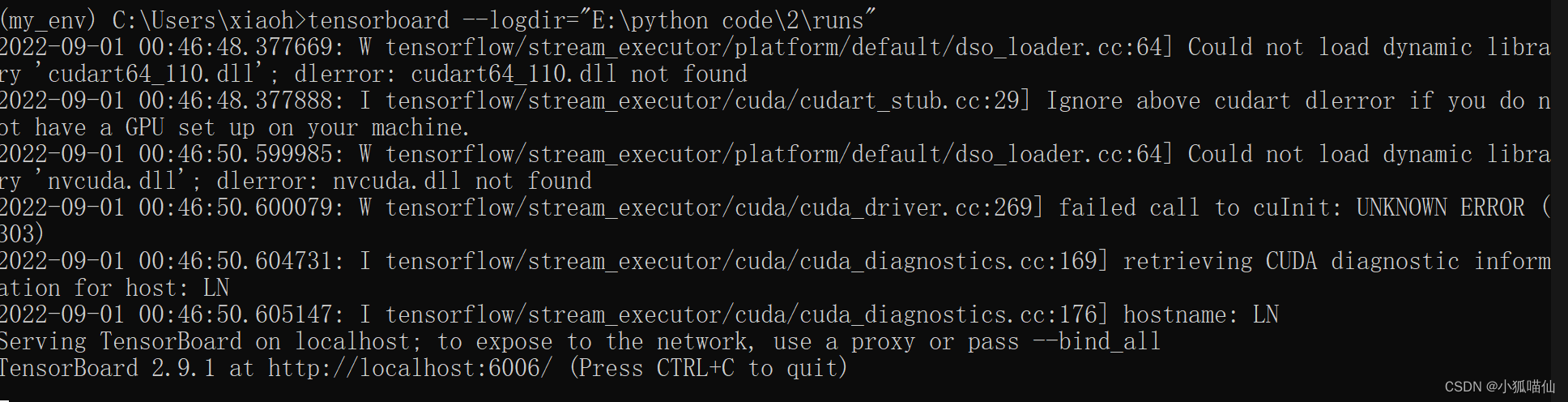

成功，复制下方网站：

tensorboard成功启动

---

图像

• 对于单张图片的显示使用add_image

• 对于多张图片的显示使用add_images

• 有时需要使用torchvision.utils.make_grid将多张图片拼成一张图片后，用writer.add_image显示

import torchvision
from torchvision import datasets, transforms
from torch.utils.data import DataLoader
​
transform_train = transforms.Compose(
    [transforms.ToTensor()])
transform_test = transforms.Compose(
    [transforms.ToTensor()])
​
train_data = datasets.CIFAR10(".", train=True, download=True, transform=transform_train)
test_data = datasets.CIFAR10(".", train=False, download=True, transform=transform_test)
train_loader = DataLoader(train_data, batch_size=64, shuffle=True)
test_loader = DataLoader(test_data, batch_size=64)
​
images, labels = next(iter(train_loader))
 
# 仅查看一张图片
writer = SummaryWriter('./pytorch_tb')
writer.add_image('images[0]', images[0])
writer.close()
 
# 将多张图片拼接成一张图片，中间用黑色网格分割
# create grid of images
writer = SummaryWriter('./pytorch_tb')
img_grid = torchvision.utils.make_grid(images)
writer.add_image('image_grid', img_grid)
writer.close()
 
# 将多张图片直接写入
writer = SummaryWriter('./pytorch_tb')
writer.add_images("images",images,global_step = 0)
writer.close()

依次运行上面三组可视化（注意不要同时在notebook的一个单元格内运行），得到的可视化结果如下（最后运行的结果在最上面）：

参数

TensorBoard可以用来可视化连续变量（或时序变量）的变化过程，通过add_scalar实现：

writer = SummaryWriter('./pytorch_tb')
for i in range(500):
    x = i
    y = x**2
    writer.add_scalar("x", x, i) #日志中记录x在第step i 的值
    writer.add_scalar("y", y, i) #日志中记录y在第step i 的值
writer.close()
writer1 = SummaryWriter('./pytorch_tb/x')
writer2 = SummaryWriter('./pytorch_tb/y')
for i in range(500):
    x = i
    y = x*2
    writer1.add_scalar("same", x, i) #日志中记录x在第step i 的值
    writer2.add_scalar("same", y, i) #日志中记录y在第step i 的值
writer1.close()
writer2.close()

当我们需要对参数（或向量）的变化，或者对其分布进行研究时，可以方便地用TensorBoard来进行可视化，通过add_histogram实现。

import torch
import numpy as np
​
# 创建正态分布的张量模拟参数矩阵
def norm(mean, std):
    t = std * torch.randn((100, 20)) + mean
    return t
 
writer = SummaryWriter('./pytorch_tb/')
for step, mean in enumerate(range(-10, 10, 1)):
    w = norm(mean, 1)
    writer.add_histogram("w", w, step)
    writer.flush()
writer.close(