


Machine Learning by Andrew Ng
💡 吴恩达机器学习课程学习笔记——Week 3
🐠 本人学习笔记汇总 合订本
✓ 课程网址 standford machine learning
🍭 参考资源
学习提纲
- Classification and Regression
- Logistic Regression Model
- Multi-class Classification
- Solving the Problem of Overfitting
Classification and Regression
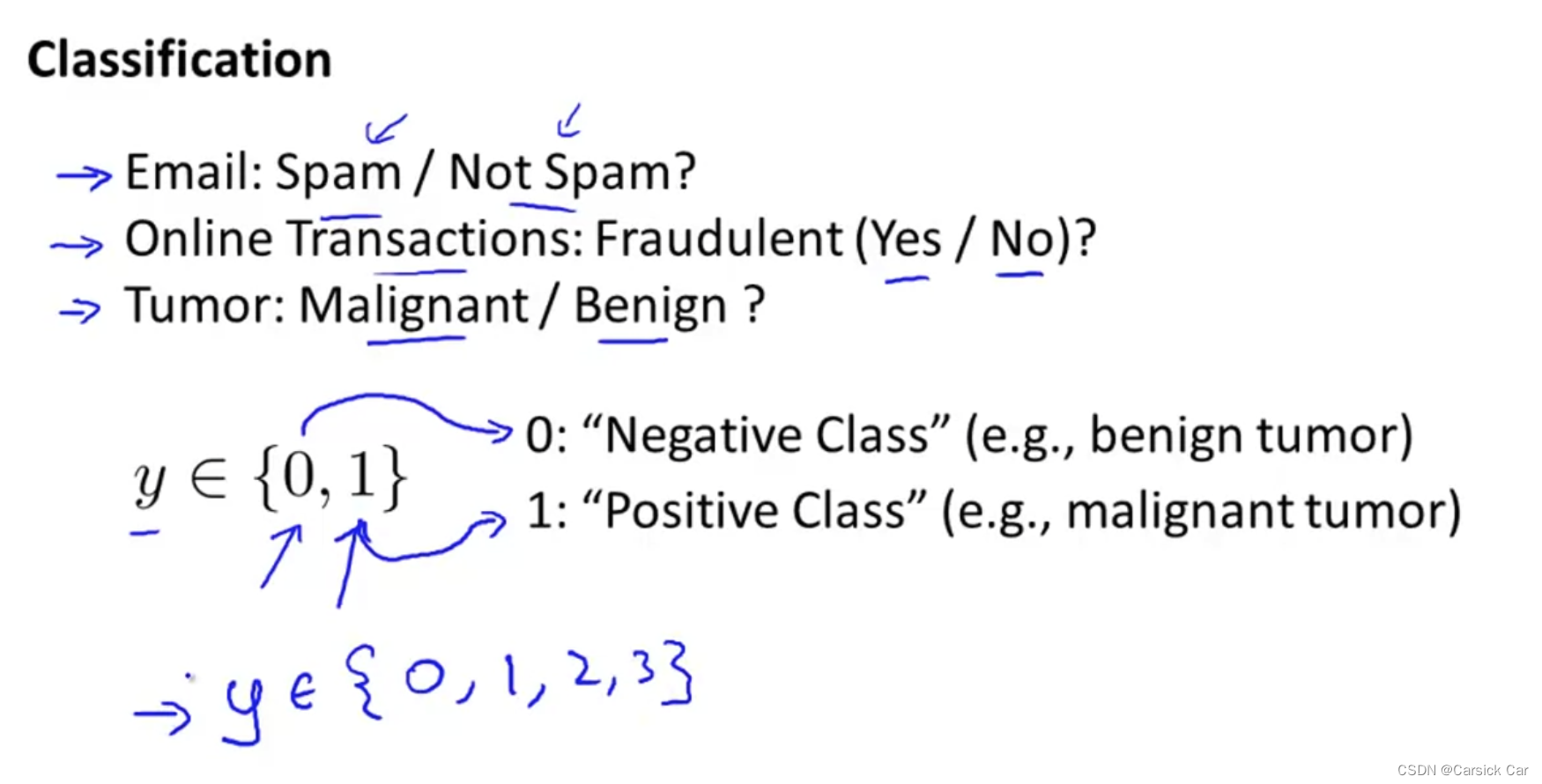
1.Classification
label 0 denotes the negative class (the absence of sth)
label 1 denotes the positive class(the presence of sth)
but it is rather arbitrary to decide which label denotes the negative/positive class
Linear Regression is not a good idea as the values to predict take on a small number of discrete values and linear regression would exceed those values.
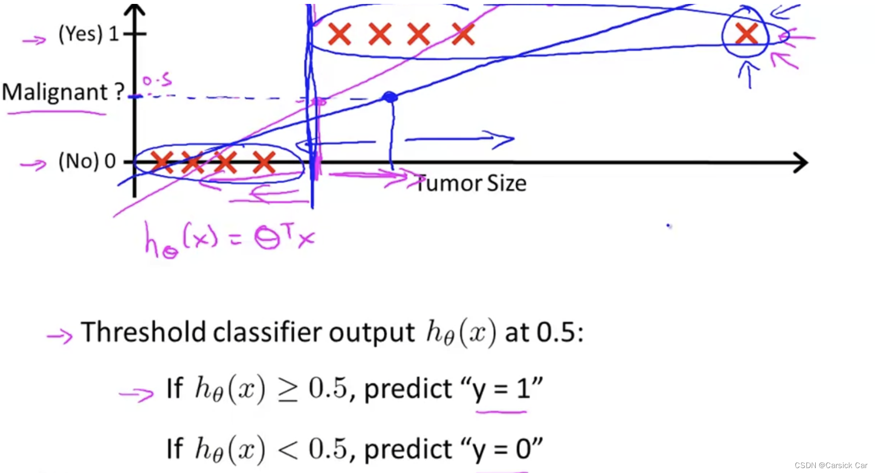
Logistic Regression is a classification algorithm 分类算法
(not a regression algorithm as its name may indicate)
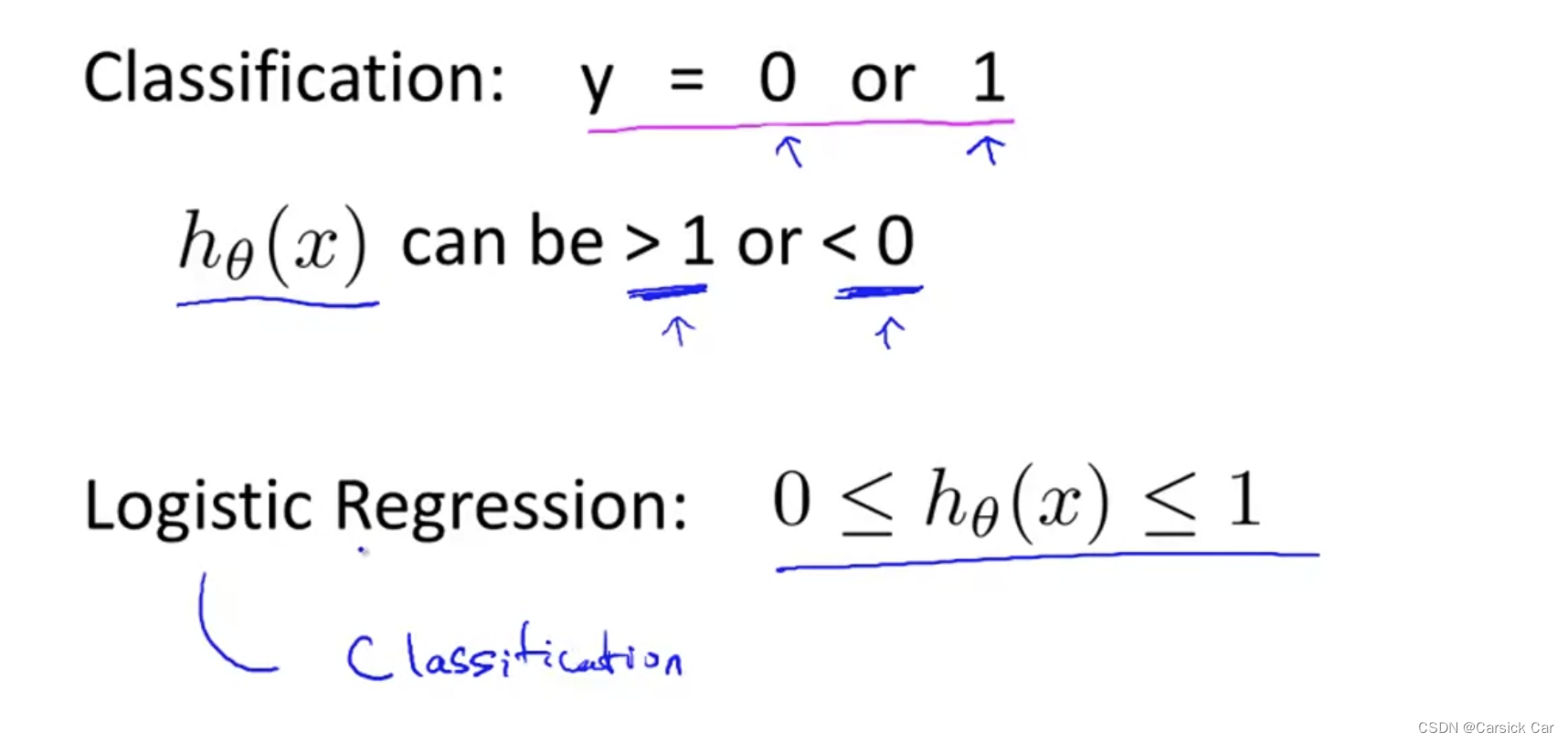
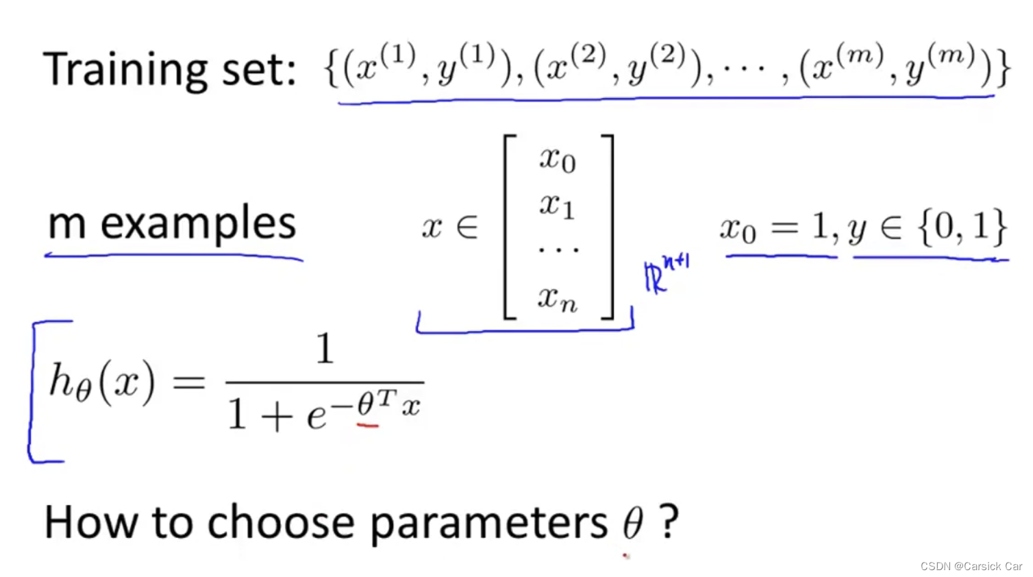
2.Hypothesis Representation
we want our classifier
0
≤
h
θ
(
x
)
≤
1
0 \le h_\theta(x) \le 1
0≤hθ(x)≤1
we turn the linear regression function
h
θ
=
θ
T
x
h_\theta = \theta^T x
hθ=θTx
into
h
θ
=
g
(
θ
T
x
)
h_\theta = g(\theta^T x)
hθ=g(θTx)
where g is
g
(
z
)
=
1
1
+
e
−
z
g(z)= \frac{1}{1+e^{-z}}
g(z)=1+e−z1
then we get
h
θ
=
1
1
+
e
−
θ
T
x
h_\theta = \frac{1}{1+e^{-{\theta^T x}}}
hθ=1+e−θTx1
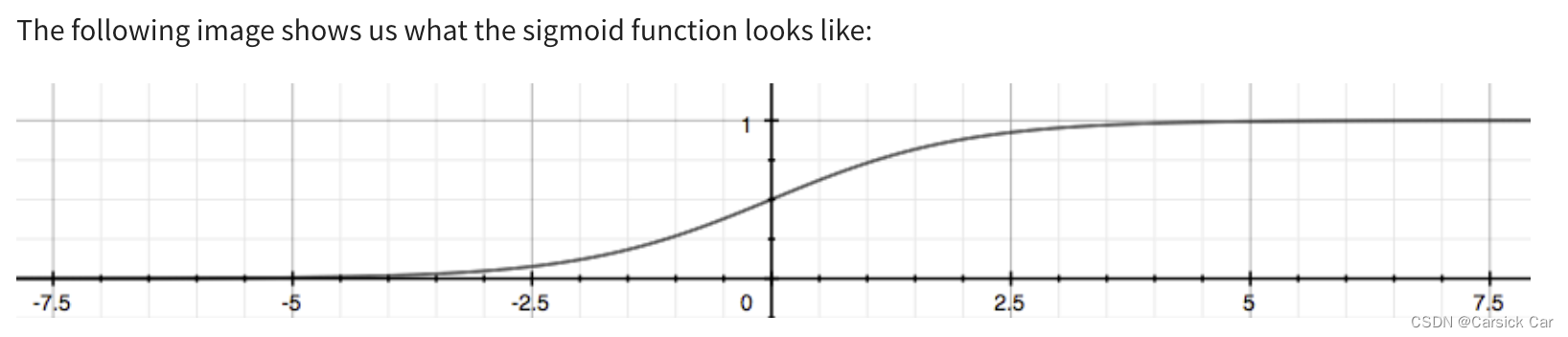
g is called sigmoid function or logistic function。
Sigmoid函数的性质:
g asymptotes at 0 as z goes to minus infinity, g asymptotes at 1 as z goes to infinity
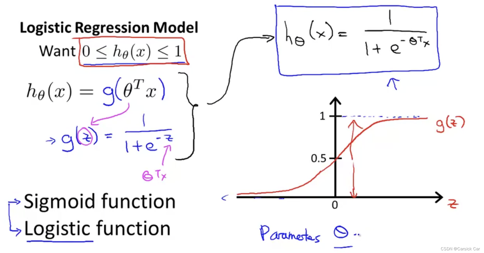
The look of the sigmoid function 函数曲线
malignant 恶性 benign 良性
Interpretation of Hypothesis Output 解读假设函数的输出
The probability that y = 1, given x, parameterized by
θ
\theta
θ 在
θ
\theta
θ参数下,给定x,y=1的概率
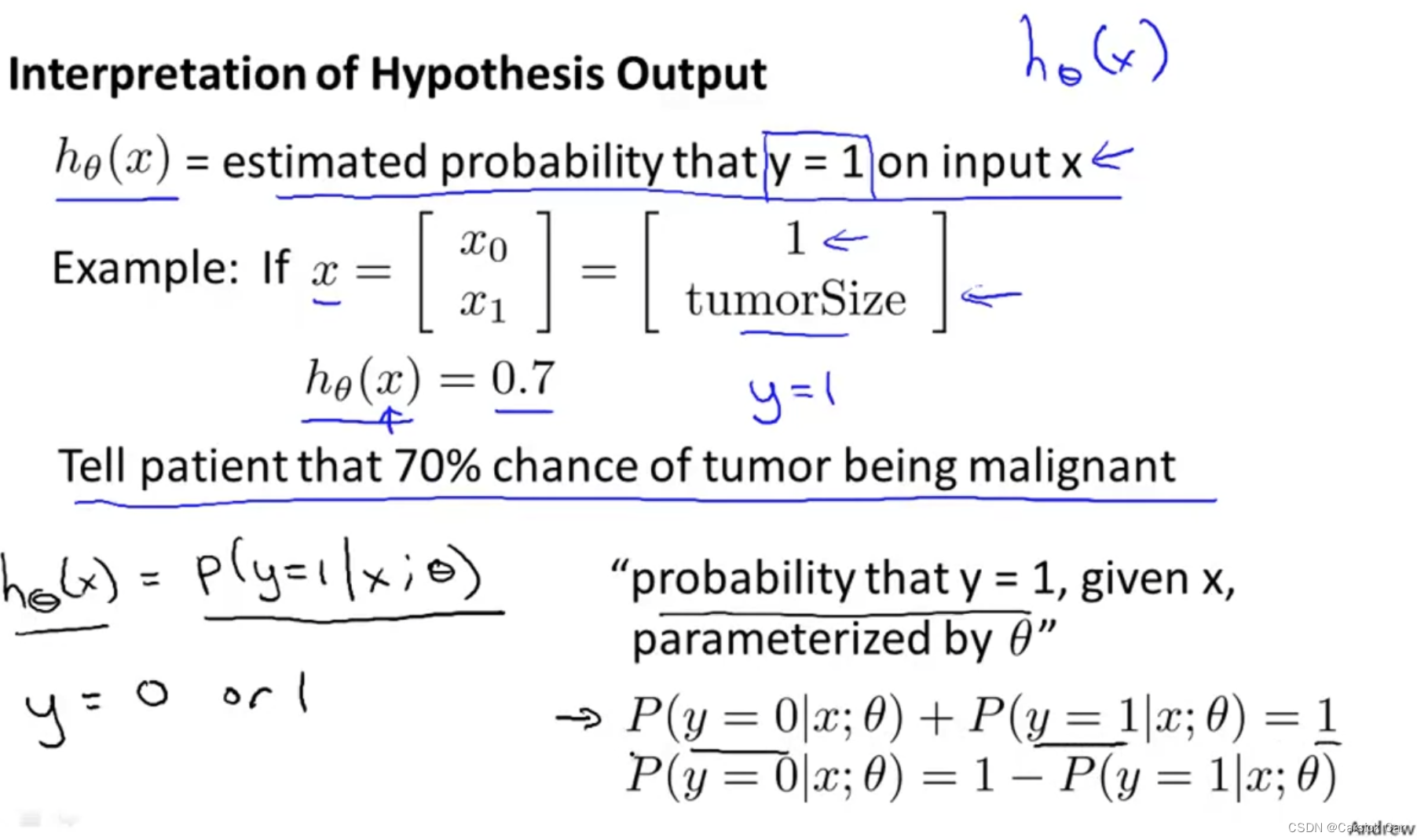
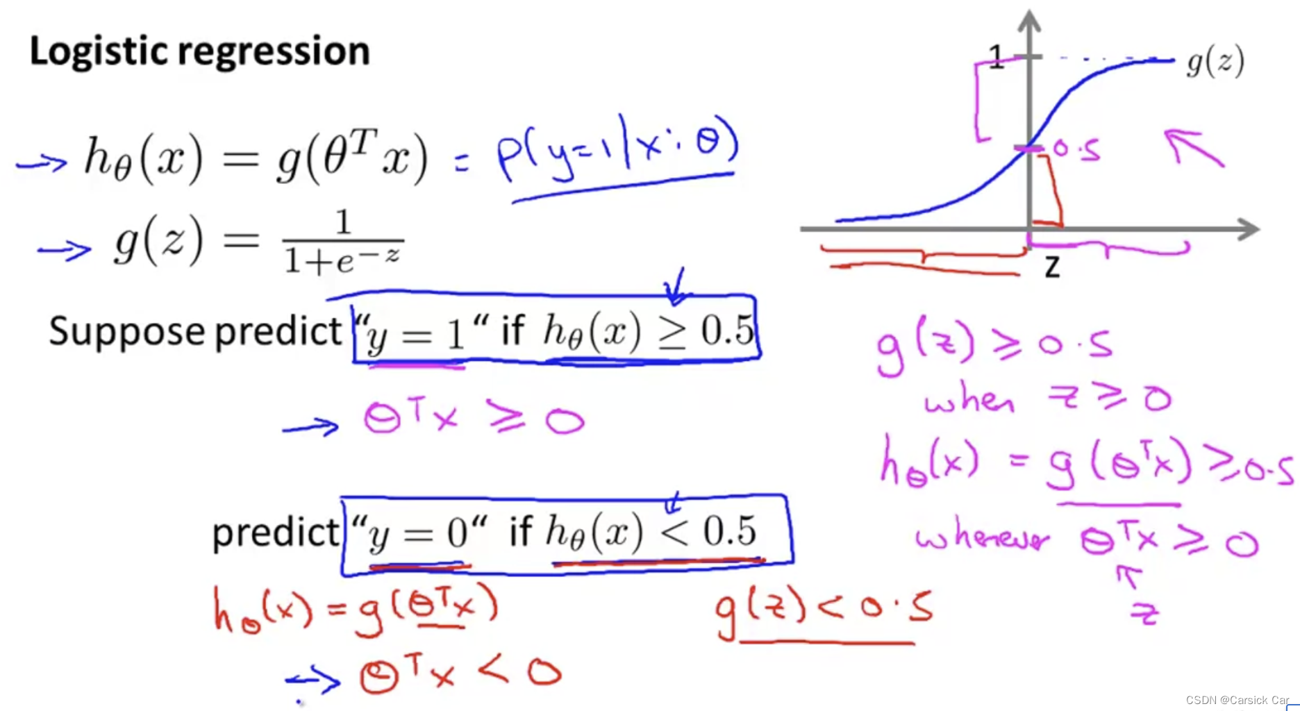
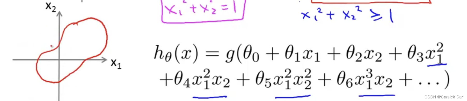
3.Decision Boundary 决策边界
The Decision Boudary
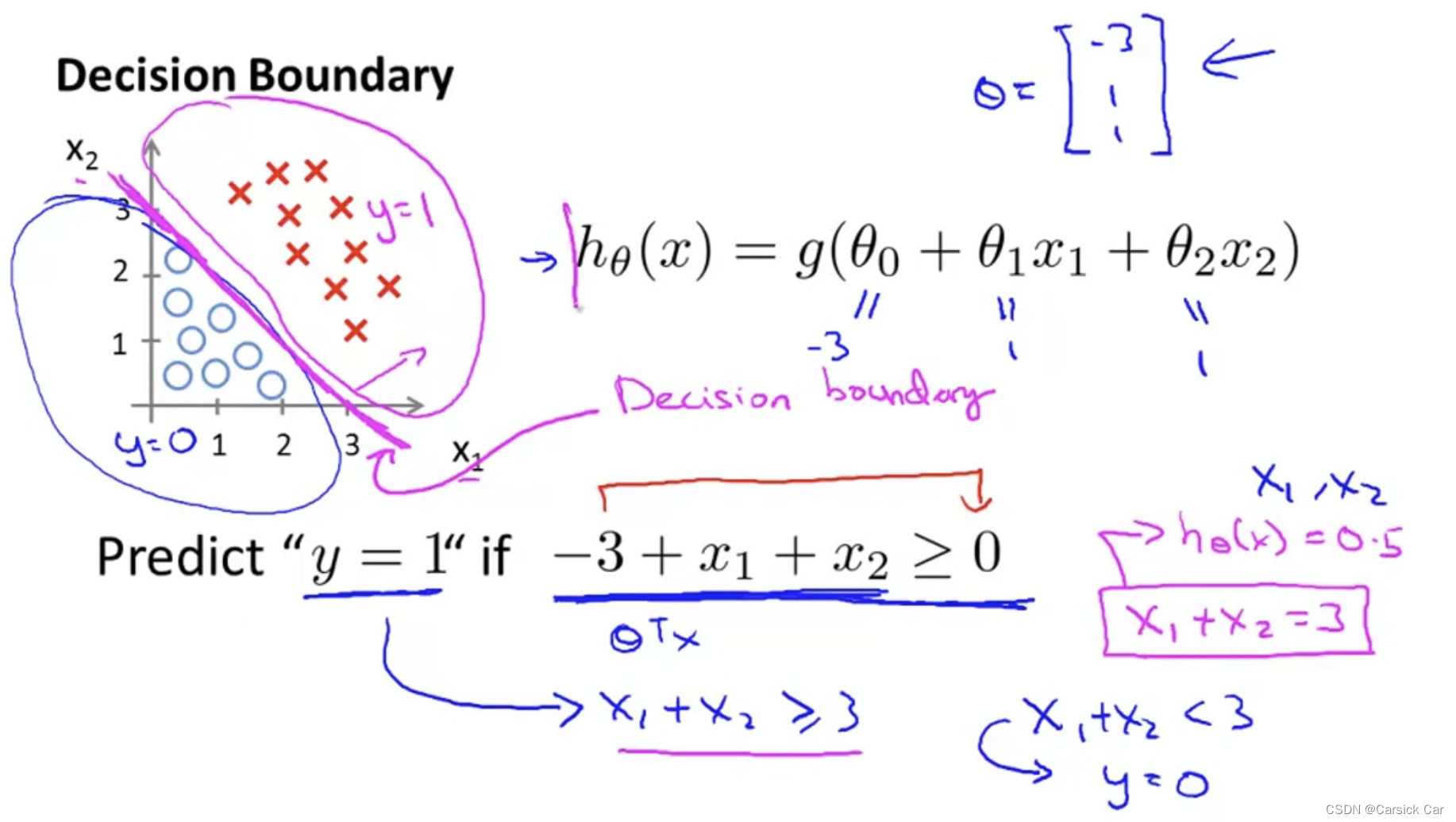
The boundary is decided by parameters, not the training set

with more higher order polynomial terms, we can get more complex decision boundaries
通过构造高阶多项式函数,我们可以得到更加复杂的决策边界。
Logistic Regression Model
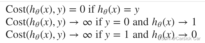
1.Cost Function
= optimization objective 优化目标
Given a training set, how to choose
θ
\theta
θ
comma 逗号 ,
Cost function of linear regression
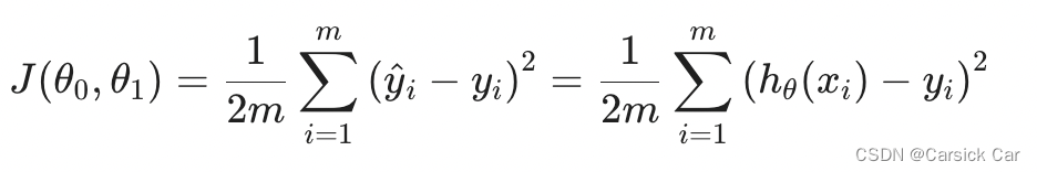
if we directly use the cost function of linear regression, it turn out to be a non-convex function. 不能直接套用线性回归的损失函数,因为用于分类问题的话,它是非凸的。
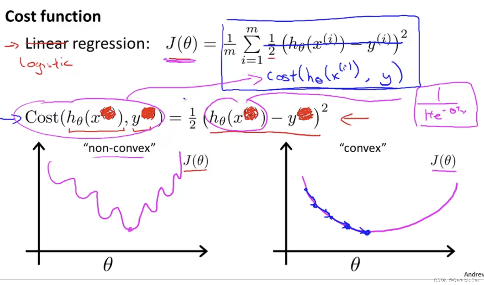
so, we have to find a new const function to make J convex
J ( θ ) = 1 m Σ i = 1 m C o s t ( h θ ( x i , y ) ) J(\theta) = \frac{1}{m} \Sigma_{i=1}^m Cost(h_\theta(x^i, y)) J(θ)=m1Σi=1mCost(hθ(xi,y))
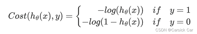
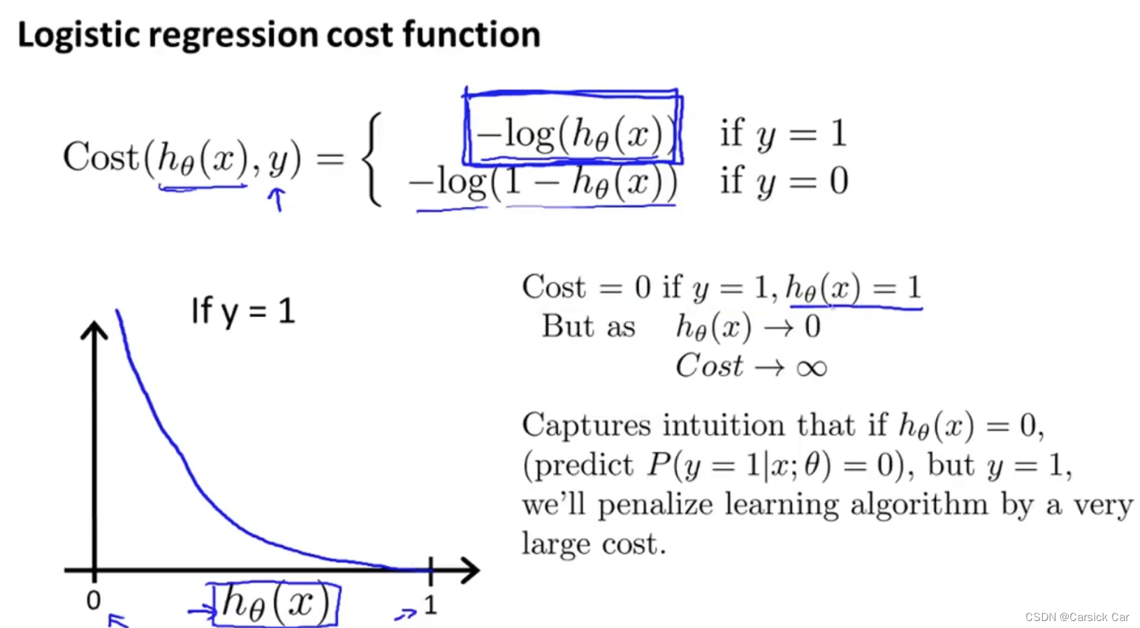
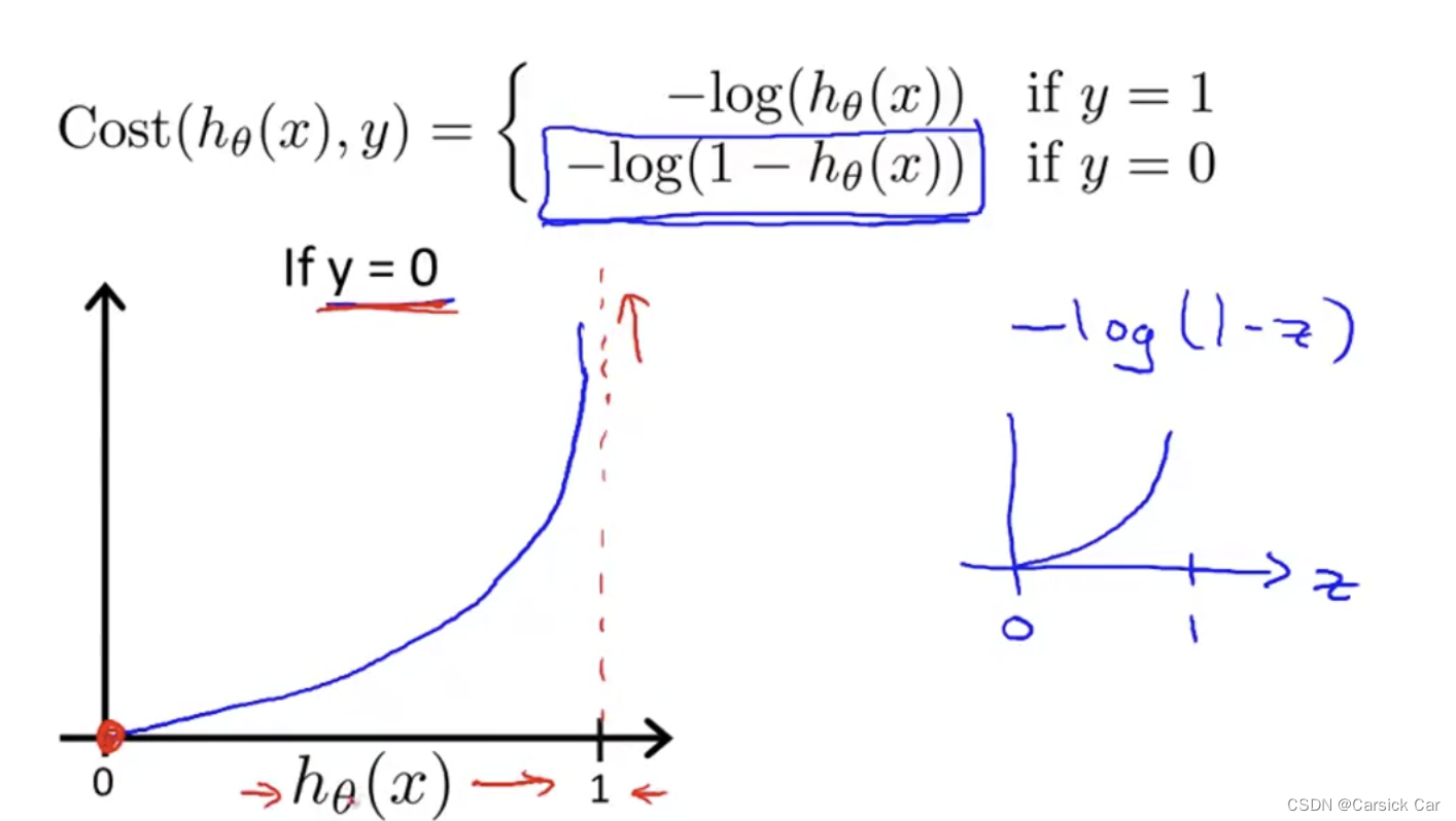
损失函数的性质:
2.Simplified Cost Function and Gradient Descent
We can compress the cost function’s two conditional cases in to one case
C
o
s
t
(
h
θ
(
x
)
,
y
)
=
−
y
l
o
g
(
h
θ
(
x
)
)
−
(
1
−
y
)
l
o
g
(
1
−
h
θ
(
x
)
)
Cost(hθ(x),y)=−ylog(hθ(x))−(1−y)log(1−hθ(x))
Cost(hθ(x),y)=−ylog(hθ(x))−(1−y)log(1−hθ(x))
The full const function
J
(
θ
)
=
−
1
m
∑
i
=
1
m
[
y
(
i
)
log
(
h
θ
(
x
(
i
)
)
)
+
(
1
−
y
(
i
)
)
log
(
1
−
h
θ
(
x
(
i
)
)
)
J(\theta) = - \frac{1}{m} \displaystyle \sum_{i=1}^m [y^{(i)}\log (h_\theta (x^{(i)})) + (1 - y^{(i)})\log (1 - h_\theta(x^{(i)}))
J(θ)=−m1i=1∑m[y(i)log(hθ(x(i)))+(1−y(i))log(1−hθ(x(i)))
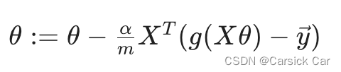
A vectorized implementation is
h
=
g
(
X
θ
)
h=g(Xθ)
h=g(Xθ)
J
(
θ
)
=
1
m
⋅
(
−
y
T
l
o
g
(
h
)
−
(
1
−
y
)
T
l
o
g
(
1
−
h
)
)
J(θ)=\frac{1}{m}⋅(−y^Tlog(h)−(1−y)^Tlog(1−h))
J(θ)=m1⋅(−yTlog(h)−(1−y)Tlog(1−h))

apply the template of gradient descent and take the the derivative of J
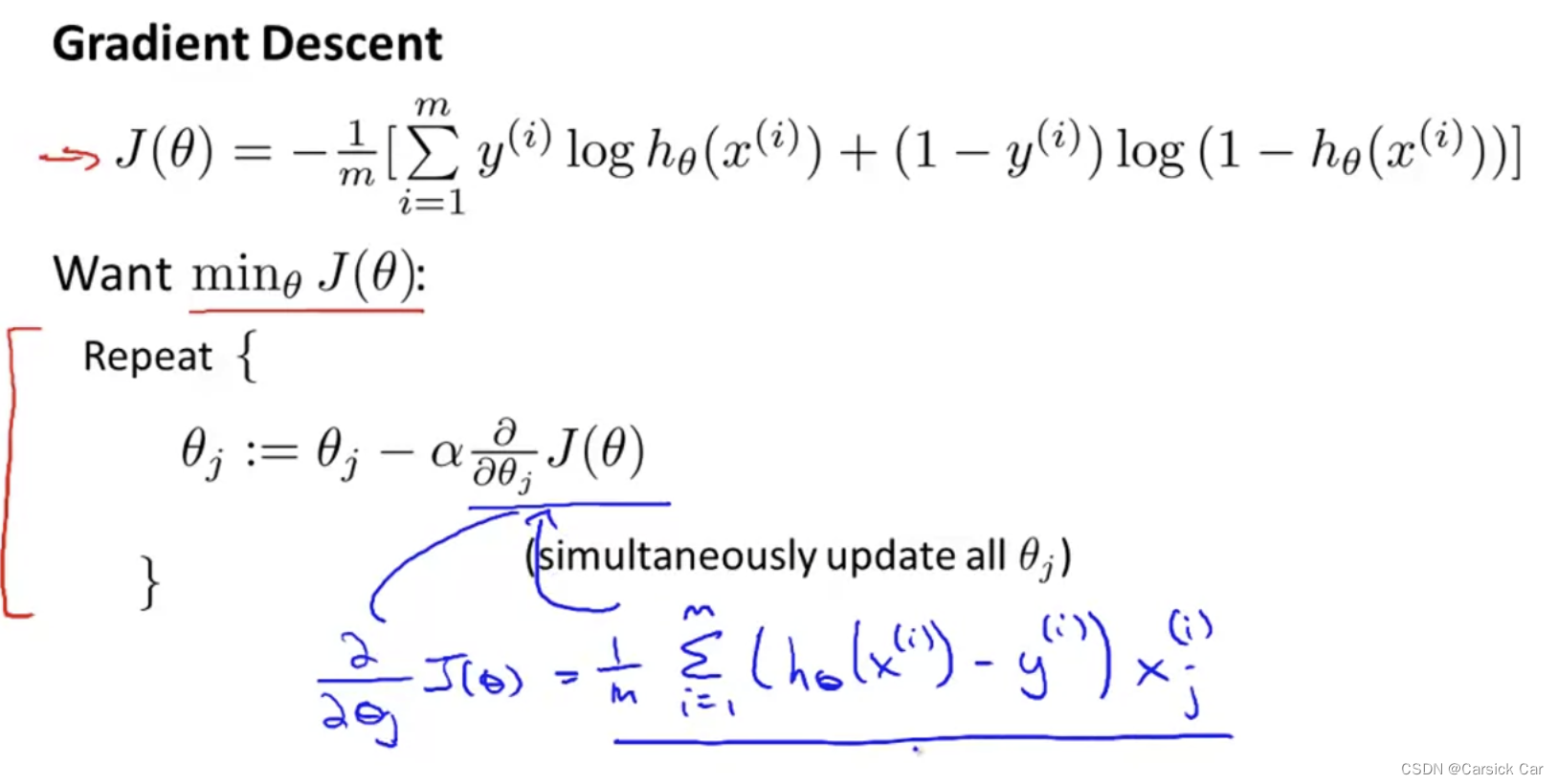
The look is identical to linear regression except that the definition of
h
θ
(
x
)
h_\theta (x)
hθ(x) is changed
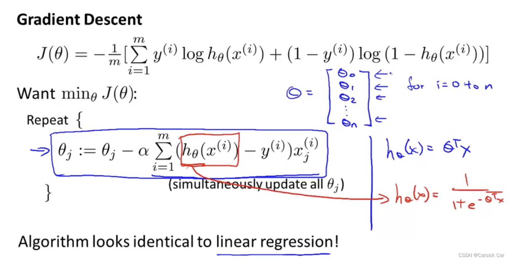
A vectorized implementation
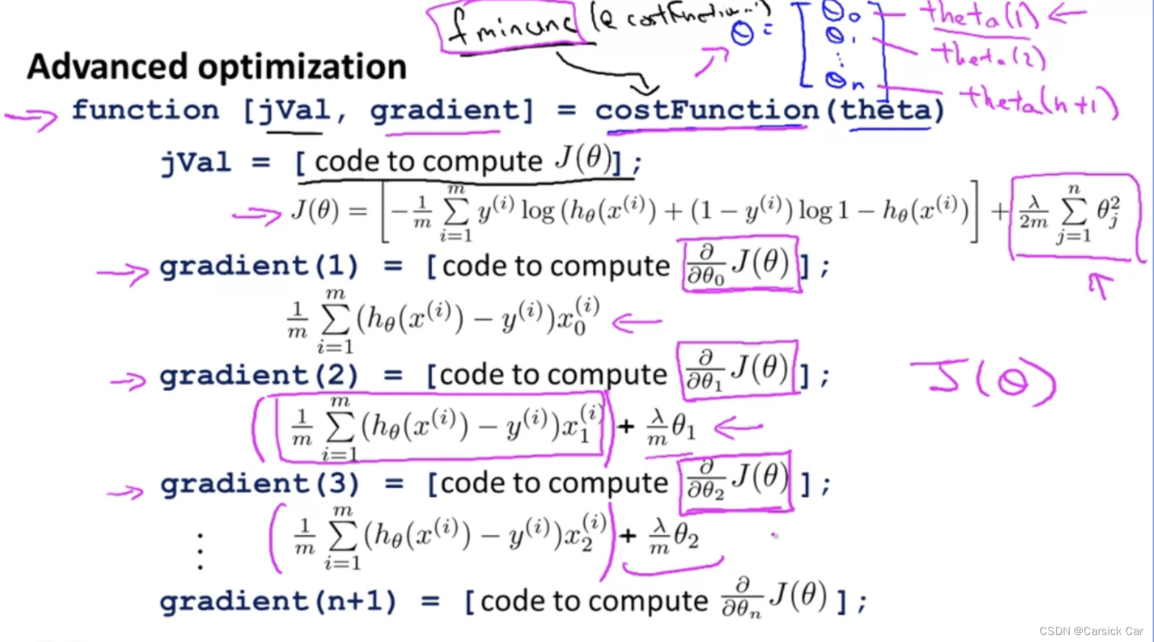
3.Advanced Optimization
There are some other optimization algorithm
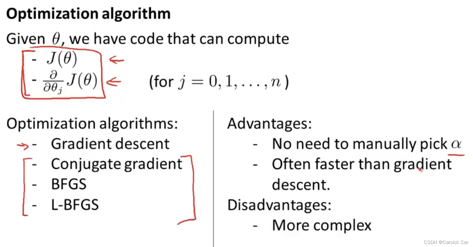
Octave part of optimization, skip
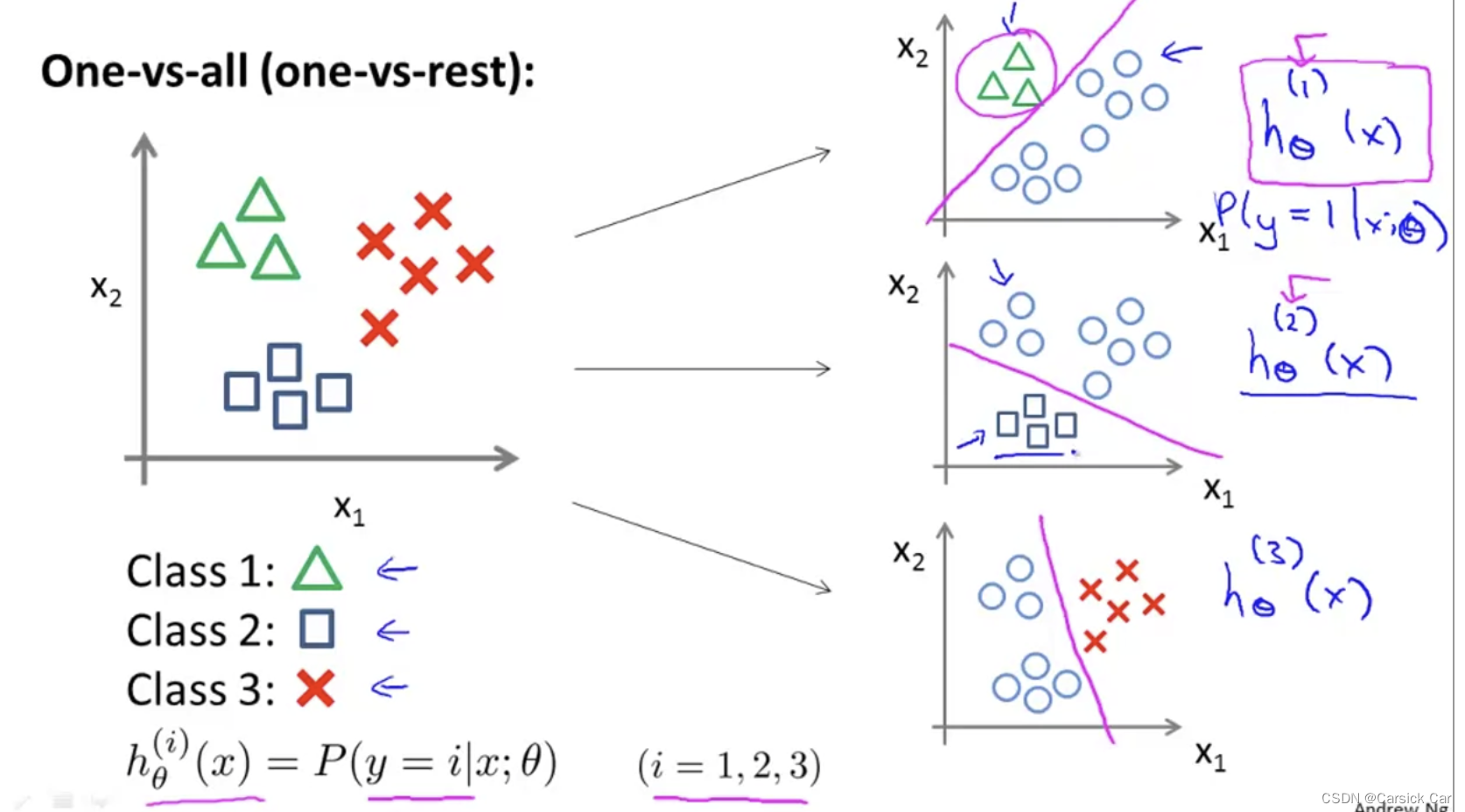
Multi-class Classification
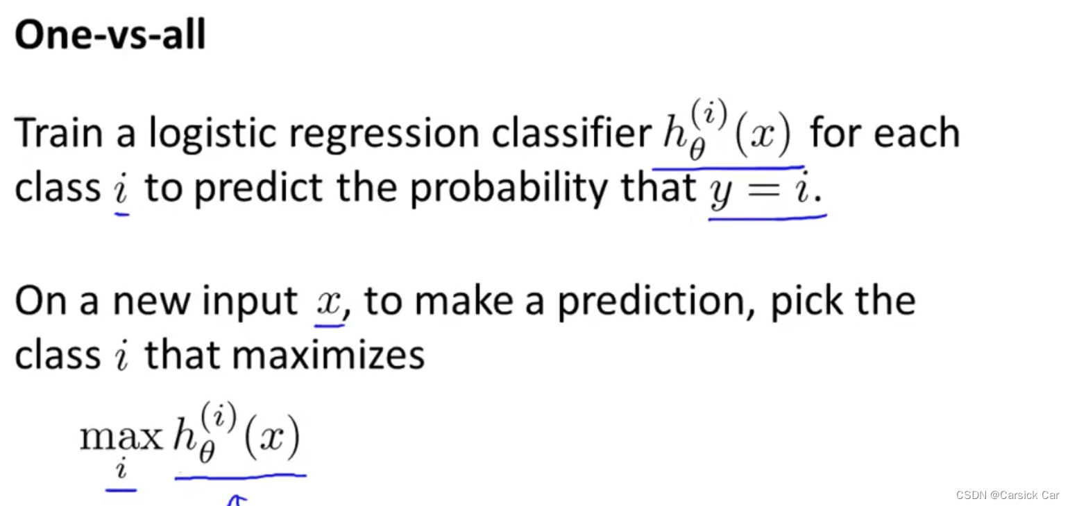
1.Multi-class Classification: 1 vs. all
Summary
use k classifiers to solve k-class problems
Solving the Problem of Overfitting
1.The Problem of Overfitting
过拟合问题:fit perfect on the training examples but bot good on the testing examples
left plot: underfitting
right plot: overfitting
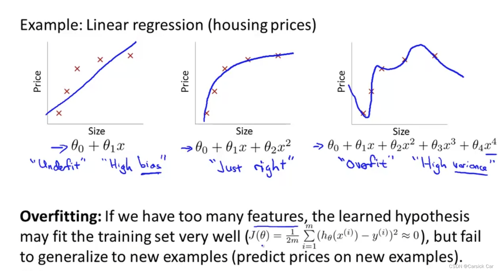
Address overfitting
- 减少特征
- 正则(下讲)

2.Cost Function
θ
0
+
θ
1
x
1
+
θ
2
x
2
+
θ
3
x
3
+
θ
4
x
4
θ_0+θ_1x_1+θ_2 x_2+θ_3x_3+θ_4x_4
θ0+θ1x1+θ2x2+θ3x3+θ4x4
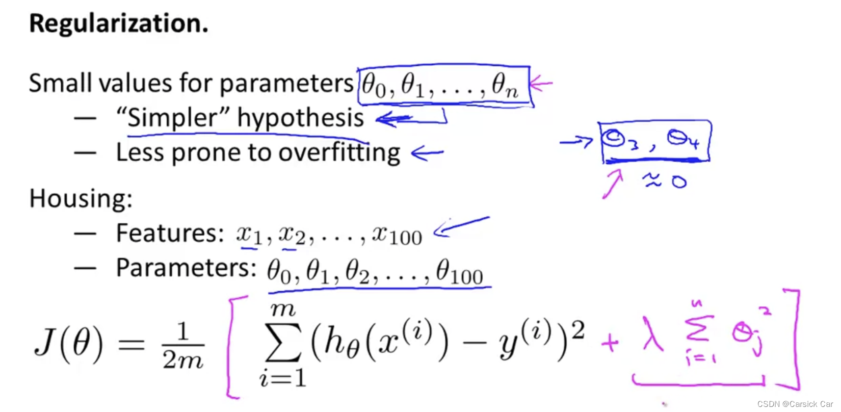
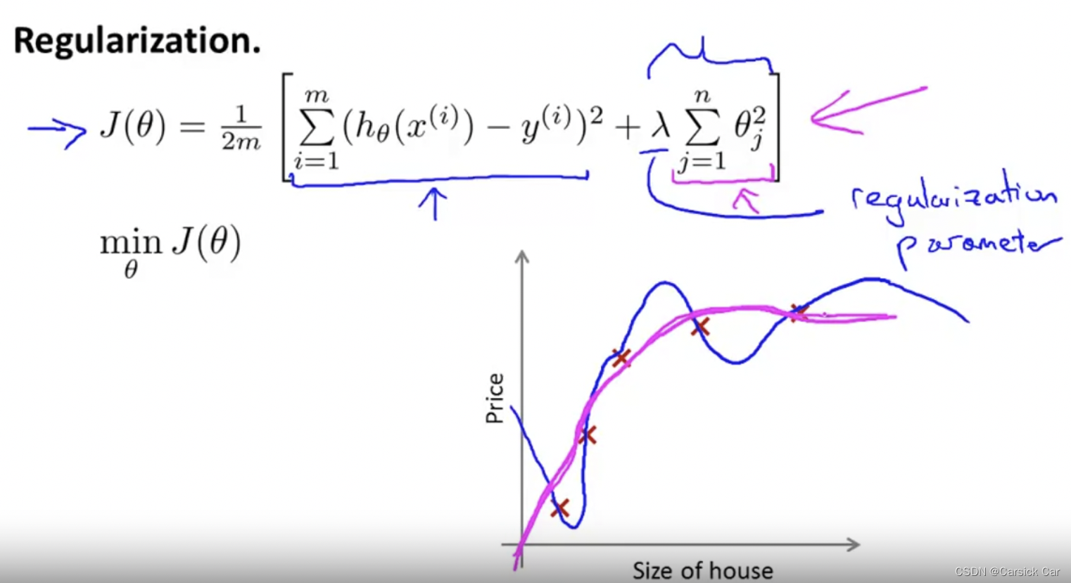
suppose we penalize and make θ3 and θ4 smaller, then we actually force to model to ‘simplify’ itself
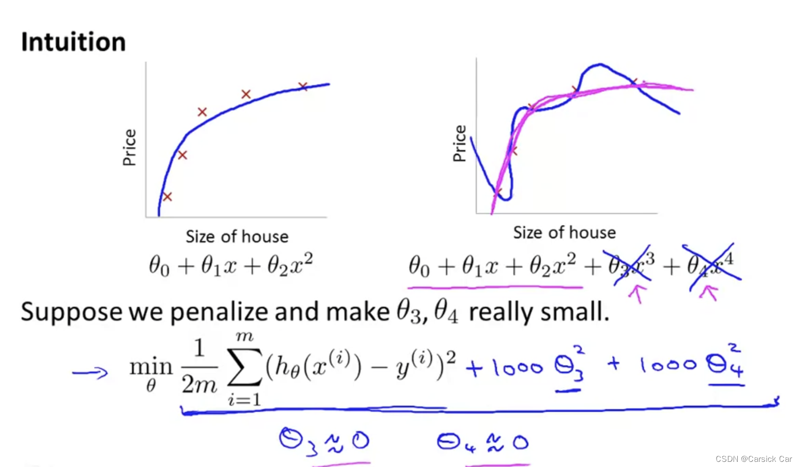
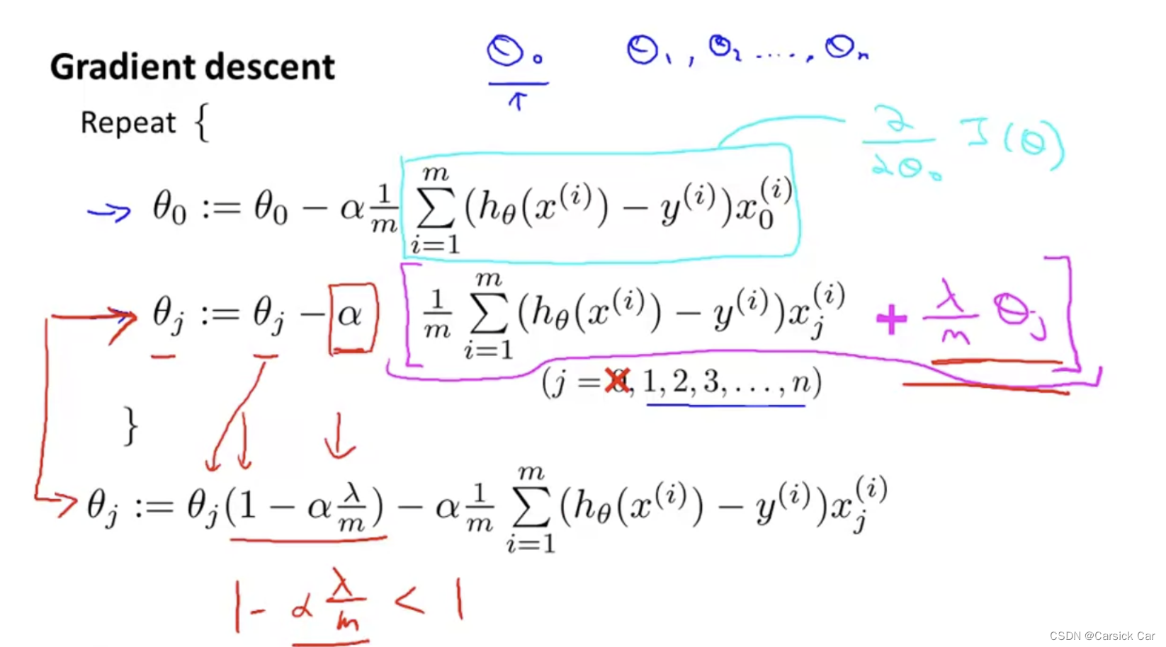
Regularization
by convention it starts from θ1 (but it makes little difference if it starts from θ0)
λ
\lambda
λ is called regularization parameter 正则参数
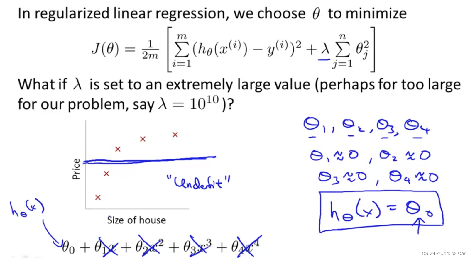
if
λ
\lambda
λ is set to an extremely large value, then all
θ
\theta
θs will be 0. “underfit”
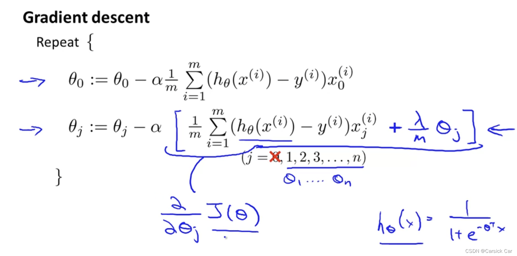
3.Regularized Linear Regression
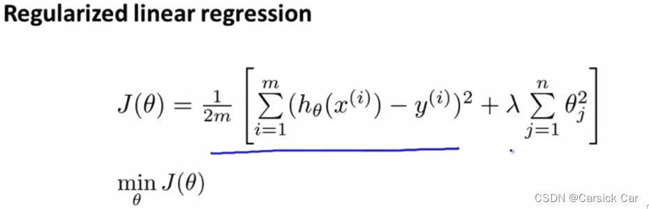
Normal Equation 中添加正则项
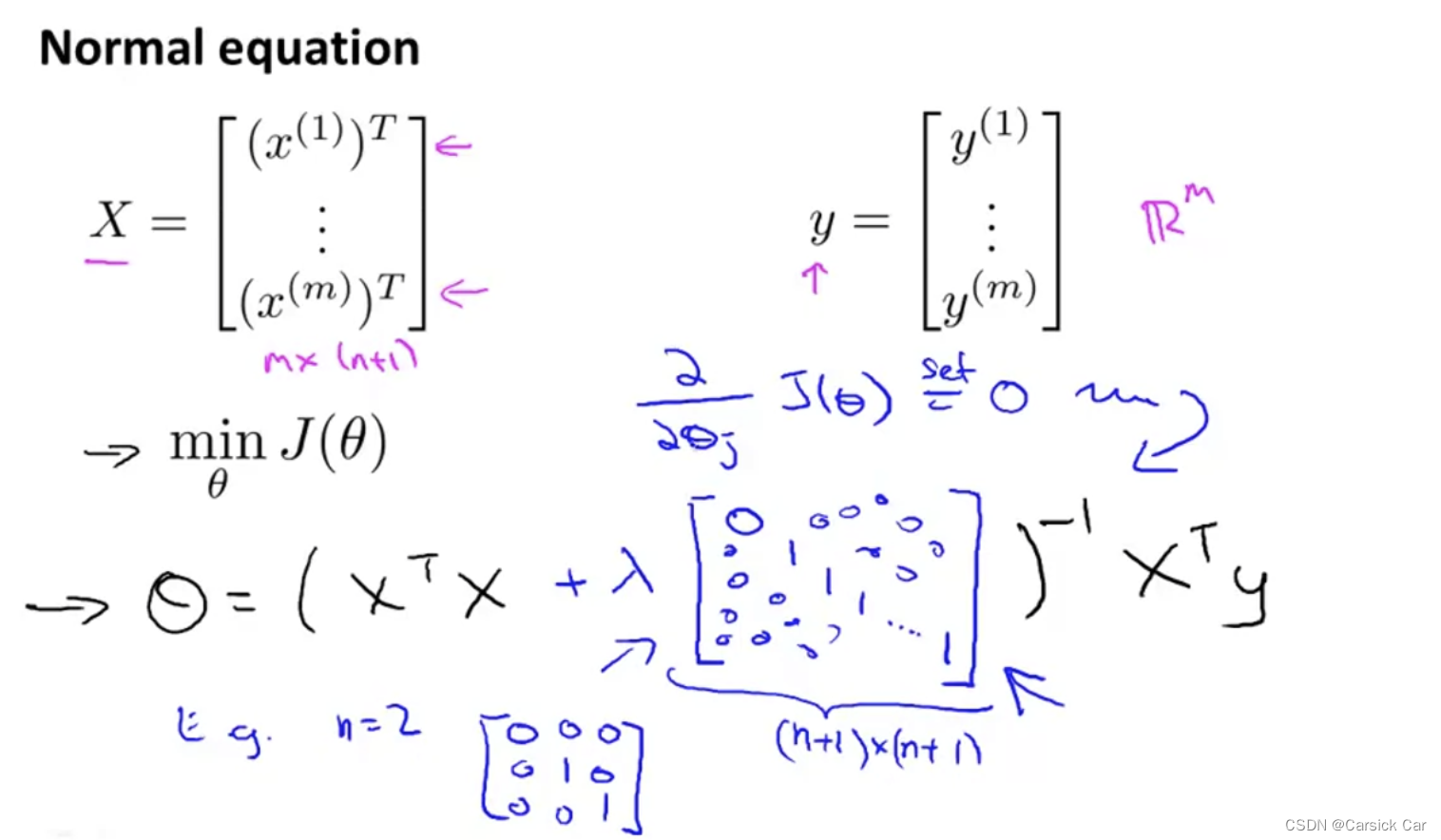
the dimension is (n + 1) * (n + 1)
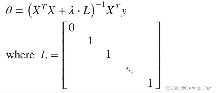
when m < n, X T X X^TX XTX is not invertible. But after adding the term λ \lambda λ * L, it becomes invertible!
4.Regularized Logistic Regression
We can regularize logistic regression in a similar way that we regularize linear regression.
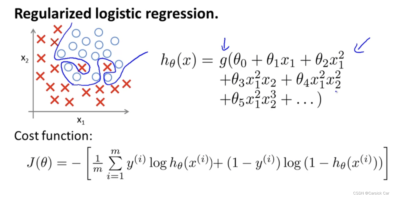
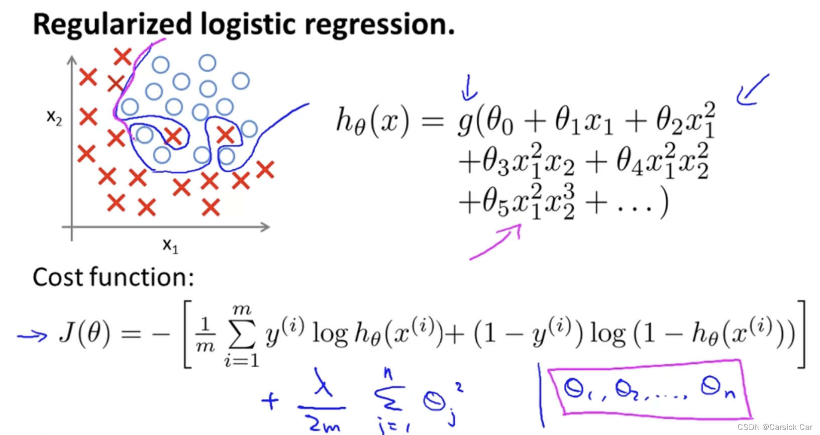
Recall that our cost function for logistic regression was:
J ( θ ) = − m 1 ∑ i = 1 m [ y i l o g ( h θ ( x i ) ) + ( 1 − y i ) l o g ( 1 − h θ ( x i ) ) ] J(θ)=−m_1∑_{i=1}^m[y^i log(h_θ(x^i))+(1−y^i) log(1−h_θ(x^i))] J(θ)=−m1∑i=1m[yilog(hθ(xi))+(1−yi)log(1−hθ(xi))]
regularize the equation
J ( θ ) = − 1 m ∑ i = 1 m [ y i l o g ( h θ ( x i ) ) + ( 1 − y i ) l o g ( 1 − h θ ( x i ) ) ] + λ 2 m ∑ j = 1 n θ j 2 J(θ)=−\frac{1}{m}∑_{i=1}^m[y^i log(h_θ(x^i))+(1−y^i) log(1−h_θ(x^i))] +\frac{λ}{2m}∑_{j=1}^nθ_j^2 J(θ)=−m1∑i=1m[yilog(hθ(xi))+(1−yi)log(1−hθ(xi))]+2mλ∑j=1nθj2
Advanced optimization


 1381
1381


 被折叠的 条评论
为什么被折叠?
被折叠的 条评论
为什么被折叠?
 到【灌水乐园】发言


