


目录
无监督学习1--聚类
什么是无监督学习?
训练集只有x1,x2...,xi,没有标签y的数据。
我们要将无标签的数据输入,然后让算法找到一些隐含在数据中的结构,
把这些无标签的数据分成一簇一簇的,就是聚类算法(学习的第一个无监督学习的算法)。
聚类有哪些应用?

K-means算法
语言表述步骤
给定一组未加标签的数据集,希望有一个算法能够自动的讲这些数据分成有紧密关系的子集或簇。
K-means算法 是目前比较热门,应用较多的算法之一。
K-mean步骤:假如下图我想把数据分成两个簇
首先随机生成两点,这两点叫做聚类中心,K-means是一个迭代算法,做两件事:第一件 簇分配,第二个 移动聚类中心。簇分类时:需要遍历每个数据,根据它与两个随机点的距离那个近,就把这个数据分配给那个点。移动聚类中心:找到所有同颜色的点计算其均值的位置为新的聚类中心。然后再次计算每个点距离中心点的距离分,重复这两个步骤,直到中心点不再改变。


伪代码表示k-means的过程
说明:假设uk是某个簇的均值,如果存在一个没有点的聚类中心,直接移除这个聚类中心,最终会得到K-1个簇;如果想要最终的到K个簇,那么需要重新初始化聚类中心;但最常见的做法,一般是直接移除。


常应用来解决分离不佳的簇的问题
 例如将根据体重设计衣服的尺寸(S,L,M)
优化目标
K:表示簇的数量;k:表示聚类中心点的下标,c^i:表示xi被划分到第几个簇。
K-means的代价函数为下图中的J,算法最终要找到c^i,μ_i,即能最小化J的参数值。这个代价函数有时也叫做 失真代价函数 或 K-means的失真。 J->畸变函数

随机初始化
如何使算法避免局部最优解?
 初始化点不同,结果也不同。
初始化选择的点可能会使结果陷入局部最优,如下图右下角两张图所示。

要避免陷入局部最优,我们需要做多次初始化而不是一次。来保证最终得到的是最优的。
常见的初始化次数在 50到1000次。当然如果K比较小,次数少一些。
选取聚类数量
目前还没有可以自动选择聚类的数目的算法,需要通过可视化数据或观察聚类的输出来选择(手动)
"肘部法则"
如果得到左图的曲线,是好的,但通常得到的图是右图,无法判断那个点,所以相当于啥都没做。
 因此不要期望它每次都有用。
下面仍然以衣服尺寸聚类为例:
衣服的销售量可能会帮你决定分成几类,怎样利用后续的目的决定什么样的衣服作为评价标准来选择聚类数。手动选择时,想想聚类的目的是什么?

无监督学习2--降维
目标1---数据压缩
压缩可以减小占用的空间,可以使学习算法运行的更快。

图一-->图二(将数据投影到一个平面)-->最后降到二维空间表示

目标2---可视化


PCA(也叫 主成分分析)
主成分分析问题规划1
PCA问题的公式描述
公式描述即用公式描述PCA的用途。 Principal component analysis(主成分分析)
数学证明过于复杂,因此这里没有数学证明u和z为什么可以这么用。
如下图:对于一个二维数据我们想找到一条直线,将点投影到这条直线上,它会找到一个低维平面(这里是一条直线),将点投影到这个面上,每个点与投影之间的距离叫做"投影误差",PCA会选择误差平方最小的面或线作为投影面或线,以便最小化平法投影误差。 
PCA与线性回归
首先,PCA不是线性回归,他们是两种不同的算法,他们计算的误差是不一样的,如下图所示。

主成分分析问题规划2
数据处理
无监督学习中,均值标准化过程(使每个特征具有均值为0的特点)与特征缩放(根据数据集决定)过程很相似。

计算u^(i),z的描述过程如下图,协方差用∑(大写的σ:一个协方差矩阵)表示,式子左边为协方差,右面是求和符号。svd:表示奇异值分解。不同语言找有这个功能的库就行了。


总结
进行均值归一化后为确保每一个特征都是均值为0的。根据数据范围任选特征缩放。预处理完后计算载体矩阵Sigma,通过这个方法,如果你的数据 是被给予作为一个矩阵如图中的X训练集矩阵,然后我们先得到要降维矩阵U的前k列,z=..定义了我们如何从一个特征向量x到降维的表示z。

主成分数量选择

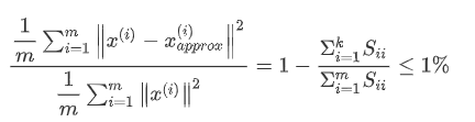
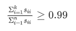
我们希望在平均 均方误差与训练集方差的比例尽可能小的情况下选择尽可能小的 k值(从n个特征降到k个特征)如果我们希望这个比例小于1%,就意味着原本数据的偏差有99%都保留下来了,如果我们选择保留90%的偏差,便能非常显著地降低模型中特征的维度了。
 我们可以先令k=1,然后进行主成分分析,获得U_{reduce}Ureduce和z,然后计算比例是否小于1%。如果不是的话再令k=2,依次类推,直到找到可以使得比例小于1%的最小k值(因为各个特征之间通常情况存在某种相关性).其中的 S是一个n×n 的矩阵,只有对角线上有值,而其它单元都是 0,我们可以使用这个矩阵来计算平均均方误差与训练集方差的比例:
即:
压缩重现
重现即怎么从压缩后的数据得到之前的数据表示?

应用PCA的建议
首先,我们尝尝使用PCA加速无监督学习算法。假设你有一个监督学习的数据,其中x^i有很高的维度,实际中这可能是一个计算机视觉的问题。即假设我们有一张 100×100 像素的图片包含10000 个像素强度值,对于这种很高维的特征向量,运行学习算法时很慢。这是用PCA降低它的维度,步骤如下:
-
首先,抽出x,不看y;运用PCA将数据压缩至1000个特征
-
然后,对训练集运行某个学习算法:逻辑回归、SVM、神经网络等
-
最后,如果有一个新的样本,将新的测试样本x经过PAC的映射关系进行映射获得相应的z,然后把z带到假设函数中
-
note:PCA定义一个从x到z的映射,这个映射只能通过在训练集上运行PCA来定义。所做的是计算一系列参数进行特征缩放和均值归一化,它还计算矩阵U_reduce(只能从训练集上训练得出)
 错误的使用PCA的情况:
 -
认为PCA是一种防止过拟合的方法。防止过拟合的最好的办法 正则化。原因在于PCA只是近似地丢弃掉一些特征,它并不考虑任何与y有关的影响,因此可能会丢失非常重要的特征。
-
默认地将PCA作为学习过程中的一部分,这虽然很多时候有效果,建议在使用PCA前先从所有原始特征开始,只在当你确定用x无法运行时(算法运行太慢或者占用太多内存)再考虑采用PCA。
-
总:PCA应用于提高算法运行效率、数据压缩、可视化。
K-means应用ex7
1.一个简单的二维数据集
import numpy as np
import pandas as pd
import matplotlib.pyplot as plt
import seaborn as sb
from scipy.io import loadmat

def find_closest_centroids(X, centroids):
    m = X.shape[0]
    k = centroids.shape[0]
    idx = np.zeros(m)

    for i in range(m):
        min_dist = 1000000
        for j in range(k):
            dist = np.sum((X[i,:] - centroids[j,:]) ** 2)
            if dist < min_dist:
                min_dist = dist
                idx[i] = j

    return idx

data = loadmat('E:/Python/machine learning/data/ex7data2.mat')
X = data['X']
initial_centroids = initial_centroids = np.array([[3, 3], [6, 2], [8, 5]])

idx = find_closest_centroids(X, initial_centroids)
idx[0:3]
array([0., 2., 1.])
data2 = pd.DataFrame(data.get('X'), columns=['X1', 'X2'])
data2.head()| X1 | X2 | |
|---|---|---|
| 0 | 1.842080 | 4.607572 |
| 1 | 5.658583 | 4.799964 |
| 2 | 6.352579 | 3.290854 |
| 3 | 2.904017 | 4.612204 |
| 4 | 3.231979 | 4.939894 |
#数据可视化
sb.set(context="notebook", style="white")
sb.lmplot('X1', 'X2', data=data2, fit_reg=False)
plt.show()
def compute_centroids(X, idx, k):
    m, n = X.shape
    centroids = np.zeros((k, n))

    for i in range(k):
        indices = np.where(idx == i)
        centroids[i,:] = (np.sum(X[indices,:], axis=1) / len(indices[0])).ravel()

    return centroids

compute_centroids(X, idx, 3)
array([[1.95399466, 5.02557006],
[3.04367119, 1.01541041],
[6.03366736, 3.00052511]])
# 将样本分配给最近的簇并重新计算簇的聚类中心
def run_k_means(X, initial_centroids, max_iters):
    m, n = X.shape
    k = initial_centroids.shape[0]
    idx = np.zeros(m)
    centroids = initial_centroids

    for i in range(max_iters):
        idx = find_closest_centroids(X, centroids)
        centroids = compute_centroids(X, idx, k)

    return idx, centroids

idx, centroids = run_k_means(X, initial_centroids, 10)

cluster1 = X[np.where(idx == 0)[0],:]
cluster2 = X[np.where(idx == 1)[0],:]
cluster3 = X[np.where(idx == 2)[0],:]

fig, ax = plt.subplots(figsize=(12,8))
ax.scatter(cluster1[:,0], cluster1[:,1], s=30, color='r', label='Cluster 1')
ax.scatter(cluster2[:,0], cluster2[:,1], s=30, color='g', label='Cluster 2')
ax.scatter(cluster3[:,0], cluster3[:,1], s=30, color='b', label='Cluster 3')
ax.legend()
plt.show()
# 创建一个选择随机样本并将其用作初始聚类中心的函数

def init_centroids(X, k):
    m, n = X.shape
    centroids = np.zeros((k, n))
    idx = np.random.randint(0, m, k)

    for i in range(k):
        centroids[i,:] = X[idx[i],:]

    return centroids

init_centroids(X, 3)
array([[3.18412176, 1.41410799],
[1.30882588, 5.30158701],
[1.95538864, 1.32156857]])
2.应用于图像压缩
这里需要暗转skimage,但直接安装会报错,需要先pip install scikit-image 这个需要等一段时间,之后再 pip install skimage,我的安装有问题。呜呜呜
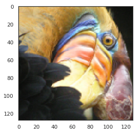
from IPython.display import Image
Image(filename='E:/Python/machine learning/data/bird_small.png')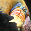
# 原始像素测像素点数值
image_data = loadmat('E:/Python/machine learning/data/bird_small.mat')
image_data
{'__header__': b'MATLAB 5.0 MAT-file, Platform: GLNXA64, Created on: Tue Jun 5 04:06:24 2012',
'__version__': '1.0',
'__globals__': [],
'A': array([[[219, 180, 103],
[230, 185, 116],
[226, 186, 110],
...,
[ 14, 15, 13],
[ 13, 15, 12],
[ 12, 14, 12]],
[[230, 193, 119],
[224, 192, 120],
[226, 192, 124],
...,
[ 16, 16, 13],
[ 14, 15, 10],
[ 11, 14, 9]],
[[228, 191, 123],
[228, 191, 121],
[220, 185, 118],
...,
[ 14, 16, 13],
[ 13, 13, 11],
[ 11, 15, 10]],
...,
[[ 15, 18, 16],
[ 18, 21, 18],
[ 18, 19, 16],
...,
[ 81, 45, 45],
[ 70, 43, 35],
[ 72, 51, 43]],
[[ 16, 17, 17],
[ 17, 18, 19],
[ 20, 19, 20],
...,
[ 80, 38, 40],
[ 68, 39, 40],
[ 59, 43, 42]],
[[ 15, 19, 19],
[ 20, 20, 18],
[ 18, 19, 17],
...,
[ 65, 43, 39],
[ 58, 37, 38],
[ 52, 39, 34]]], dtype=uint8)}
A = image_data['A']
A.shape
(128, 128, 3)
# 对数据应用一些预处理,并将其提供给K-means算法

# normalize value ranges
A = A / 255.

# reshape the array
X = np.reshape(A, (A.shape[0] * A.shape[1], A.shape[2]))
print(X.shape)

# randomly initialize the centroids
initial_centroids = init_centroids(X, 16)

# run the algorithm
idx, centroids = run_k_means(X, initial_centroids, 10)

# get the closest centroids one last time
idx = find_closest_centroids(X, centroids)

# map each pixel to the centroid value
X_recovered = centroids[idx.astype(int),:]
print(X_recovered.shape)

# reshape to the original dimensions
X_recovered = np.reshape(X_recovered, (A.shape[0], A.shape[1], A.shape[2]))
print(X_recovered.shape)
(16384, 3)
(16384, 3)
(128, 128, 3)
plt.imshow(X_recovered)
plt.show()
不知道为啥我运行出来就成黑的了
正常应该是这样的:
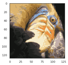
# 可以看到我们对图像进行了压缩,但图像的主要特征仍然存在
# 这就是K-means 下面我们来用scikit-learn来实现K-means
from skimage import io

# cast to float, you need to do this otherwise the color would be weird after clustring
pic = io.imread('E:/Python/machine learning/data/bird_small.png') / 255.
io.imshow(pic)
plt.show()
print(pic.shape)

# serialize data
data = pic.reshape(128*128, 3)

print(data.shape)

from sklearn.cluster import KMeans#导入kmeans库

model = KMeans(n_clusters=16, n_init=100, n_jobs=-1)

model.fit(data)
(128, 128, 3)
(16384, 3)
KMeans(algorithm='auto', copy_x=True, init='k-means++', max_iter=300,
n_clusters=16, n_init=100, n_jobs=-1, precompute_distances='auto',
random_state=None, tol=0.0001, verbose=0)
centroids = model.cluster_centers_
print(centroids.shape)

C = model.predict(data)
print(C.shape)

print(centroids[C].shape)

compressed_pic = centroids[C].reshape((128,128,3))

fig, ax = plt.subplots(1, 2)
ax[0].imshow(pic)
ax[1].imshow(compressed_pic)
plt.show()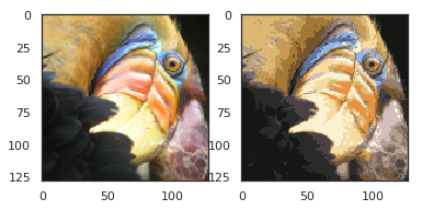
PCAex7
1.将PCA应用于一个简单的二维数据集
# PCA1
data = loadmat('E:/Python/machine learning/data/ex7data1.mat')
data
{'__header__': b'MATLAB 5.0 MAT-file, Platform: PCWIN64, Created on: Mon Nov 14 22:41:44 2011',
'__version__': '1.0',
'__globals__': [],
'X': array([[3.38156267, 3.38911268],
[4.52787538, 5.8541781 ],
[2.65568187, 4.41199472],
[2.76523467, 3.71541365],
[2.84656011, 4.17550645],
[3.89067196, 6.48838087],
[3.47580524, 3.63284876],
[5.91129845, 6.68076853],
[3.92889397, 5.09844661],
[4.56183537, 5.62329929],
[4.57407171, 5.39765069],
[4.37173356, 5.46116549],
[4.19169388, 4.95469359],
[5.24408518, 4.66148767],
[2.8358402 , 3.76801716],
[5.63526969, 6.31211438],
[4.68632968, 5.6652411 ],
[2.85051337, 4.62645627],
[5.1101573 , 7.36319662],
[5.18256377, 4.64650909],
[5.70732809, 6.68103995],
[3.57968458, 4.80278074],
[5.63937773, 6.12043594],
[4.26346851, 4.68942896],
[2.53651693, 3.88449078],
[3.22382902, 4.94255585],
[4.92948801, 5.95501971],
[5.79295774, 5.10839305],
[2.81684824, 4.81895769],
[3.88882414, 5.10036564],
[3.34323419, 5.89301345],
[5.87973414, 5.52141664],
[3.10391912, 3.85710242],
[5.33150572, 4.68074235],
[3.37542687, 4.56537852],
[4.77667888, 6.25435039],
[2.6757463 , 3.73096988],
[5.50027665, 5.67948113],
[1.79709714, 3.24753885],
[4.3225147 , 5.11110472],
[4.42100445, 6.02563978],
[3.17929886, 4.43686032],
[3.03354125, 3.97879278],
[4.6093482 , 5.879792 ],
[2.96378859, 3.30024835],
[3.97176248, 5.40773735],
[1.18023321, 2.87869409],
[1.91895045, 5.07107848],
[3.95524687, 4.5053271 ],
[5.11795499, 6.08507386]])}
X = data['X']

fig, ax = plt.subplots(figsize=(12,8))
ax.scatter(X[:, 0], X[:, 1])
plt.show()
# PCA的算法相当简单。 在确保数据被归一化之后,输出仅仅是原始数据的协方差矩阵的奇异值分解
def pca(X):
    # normalize the features
    X = (X - X.mean()) / X.std()

    # compute the covariance matrix
    X = np.matrix(X)
    cov = (X.T * X) / X.shape[0]

    # perform SVD
    U, S, V = np.linalg.svd(cov)

    return U, S, V

U, S, V = pca(X)
U, S, V
(matrix([[-0.79241747, -0.60997914],
[-0.60997914, 0.79241747]]),
array([1.43584536, 0.56415464]),
matrix([[-0.79241747, -0.60997914],
[-0.60997914, 0.79241747]]))
# 实现一个计算投影并且仅选择顶部K个分量的函数,有效地减少了维数
def project_data(X, U, k):
    U_reduced = U[:,:k]
    return np.dot(X, U_reduced)

Z = project_data(X, U, 1)
Z
matrix([[-4.74689738],
        [-7.15889408],
        [-4.79563345],
        [-4.45754509],
        [-4.80263579],
        [-7.04081342],
        [-4.97025076],
        [-8.75934561],
        [-6.2232703 ],
        [-7.04497331],
        [-6.91702866],
        [-6.79543508],
        [-6.3438312 ],
        [-6.99891495],
        [-4.54558119],
        [-8.31574426],
        [-7.16920841],
        [-5.08083842],
        [-8.54077427],
        [-6.94102769],
        [-8.5978815 ],
        [-5.76620067],
        [-8.2020797 ],
        [-6.23890078],
        [-4.37943868],
        [-5.56947441],
        [-7.53865023],
        [-7.70645413],
        [-5.17158343],
        [-6.19268884],
        [-6.24385246],
        [-8.02715303],
        [-4.81235176],
        [-7.07993347],
        [-5.45953289],
        [-7.60014707],
        [-4.39612191],
        [-7.82288033],
        [-3.40498213],
        [-6.54290343],
        [-7.17879573],
        [-5.22572421],
        [-4.83081168],
        [-7.23907851],
        [-4.36164051],
        [-6.44590096],
        [-2.69118076],
        [-4.61386195],
        [-5.88236227],
        [-7.76732508]])
# 我们也可以通过反向转换步骤来恢复原始数据。
def recover_data(Z, U, k):
    U_reduced = U[:,:k]
    return np.dot(Z, U_reduced.T)

X_recovered = recover_data(Z, U, 1)
X_recovered
matrix([[3.76152442, 2.89550838],
[5.67283275, 4.36677606],
[3.80014373, 2.92523637],
[3.53223661, 2.71900952],
[3.80569251, 2.92950765],
[5.57926356, 4.29474931],
[3.93851354, 3.03174929],
[6.94105849, 5.3430181 ],
[4.93142811, 3.79606507],
[5.58255993, 4.29728676],
[5.48117436, 4.21924319],
[5.38482148, 4.14507365],
[5.02696267, 3.8696047 ],
[5.54606249, 4.26919213],
[3.60199795, 2.77270971],
[6.58954104, 5.07243054],
[5.681006 , 4.37306758],
[4.02614513, 3.09920545],
[6.76785875, 5.20969415],
[5.50019161, 4.2338821 ],
[6.81311151, 5.24452836],
[4.56923815, 3.51726213],
[6.49947125, 5.00309752],
[4.94381398, 3.80559934],
[3.47034372, 2.67136624],
[4.41334883, 3.39726321],
[5.97375815, 4.59841938],
[6.10672889, 4.70077626],
[4.09805306, 3.15455801],
[4.90719483, 3.77741101],
[4.94773778, 3.80861976],
[6.36085631, 4.8963959 ],
[3.81339161, 2.93543419],
[5.61026298, 4.31861173],
[4.32622924, 3.33020118],
[6.02248932, 4.63593118],
[3.48356381, 2.68154267],
[6.19898705, 4.77179382],
[2.69816733, 2.07696807],
[5.18471099, 3.99103461],
[5.68860316, 4.37891565],
[4.14095516, 3.18758276],
[3.82801958, 2.94669436],
[5.73637229, 4.41568689],
[3.45624014, 2.66050973],
[5.10784454, 3.93186513],
[2.13253865, 1.64156413],
[3.65610482, 2.81435955],
[4.66128664, 3.58811828],
[6.1549641 , 4.73790627]])
fig, ax = plt.subplots(figsize=(12,8))
ax.scatter(list(X_recovered[:, 0]), list(X_recovered[:, 1]))
plt.show()
# 注意,第一主成分的投影轴基本上是数据集中的对角线。 当我们将数据减少到一个维度时,我们失去了该对角线周围的变化,
# 所以在我们的再现中,一切都沿着该对角线
2.将PCA应用于脸部图像
faces = loadmat('E:/Python/machine learning/data/ex7faces.mat')
X = faces['X']
X.shape
(5000, 1024)
def plot_n_image(X, n):
    """ plot first n images
    n has to be a square number
    """
    pic_size = int(np.sqrt(X.shape[1]))
    grid_size = int(np.sqrt(n))

    first_n_images = X[:n, :]

    fig, ax_array = plt.subplots(nrows=grid_size, ncols=grid_size,
                                    sharey=True, sharex=True, figsize=(8, 8))

    for r in range(grid_size):
        for c in range(grid_size):
            ax_array[r, c].imshow(first_n_images[grid_size * r + c].reshape((pic_size, pic_size)))
            plt.xticks(np.array([]))
            plt.yticks(np.array([]))

face = np.reshape(X[3,:], (32, 32))

plt.imshow(face)
plt.show()
# 看起来很糟糕。 这些只有32 x 32灰度的图像(它也是侧面渲染,但我们现在可以忽略)。 我们的下一步是在面数据集上运行PCA,并取得前100个主要特征。

U, S, V = pca(X)
Z = project_data(X, U, 100)

# 现在我们可以尝试恢复原来的结构并再次渲染。
X_recovered = recover_data(Z, U, 100)
face = np.reshape(X_recovered[3,:], (32, 32))
plt.imshow(face)
plt.show()
# 注意,我们失去了一些细节,尽管没有像您预期的维度数量减少10倍 


 1948
1948


 被折叠的 条评论
为什么被折叠?
被折叠的 条评论
为什么被折叠?
 到【灌水乐园】发言


