pytorch-梯度下降算法

import matplotlib.pyplot as plt

x_data=[1.0,2.0,3.0]
y_data=[2.0,4.0,6.0]

w=1.0

def forward(x):
    return x*w

def cost(xs,ys):
    cost=0
    for x,y in zip(xs,ys):
        y_pred=forward(x)
        cost+=(y_pred-y)**2
    return cost/len(xs)

   

def gradient(xs,ys):#定义得梯度函数
    grad=0
    for x,y in zip(xs,ys):
        grad+=2*x*(x*w-y)
    return grad/len(xs)
    

epoch_list=[]
loss_list=[]
print('predict  before training',4,forward(4))
for epoch in range(100):
    cost_val=cost(x_data,y_data)
    grad_val=gradient(x_data,y_data)
    w=w-0.01*grad_val
    print('progress',epoch,'w=',w,'loss',cost_val)
    epoch_list.append(epoch)
    loss_list.append(cost_val)

print('predict after training',4,forward(4))
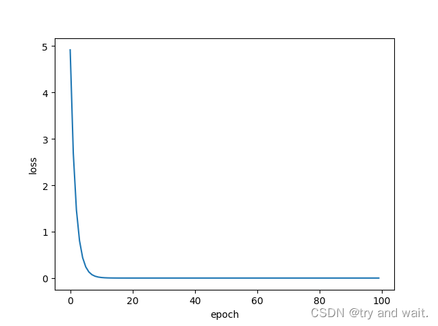
plt.plot(epoch_list,loss_list)
plt.xlabel('epoch')
plt.ylabel('loss')
plt.show()

import matplotlib.pyplot as plt

x_data=[1.0,2.0,3.0]
y_data=[2.0,4.0,6.0]

w=1.0

def forward(x):
    return x*w

def loss(x,y):
    y_pred=forward(x)
    return (y_pred-y)**2

def gradient(x,y):#定义得梯度函数
    return 2*x*(x*w-y)

epoch_list=[]
loss_list=[]
print('predict  before training',4,forward(4))
for epoch in range(100):
    for x,y in zip(x_data,y_data):
        grad=gradient(x,y)
        w=w-0.01*grad
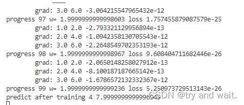
        print('\tgrad:',x,y,grad)
        l=loss(x,y)
    print('progress',epoch,'w=',w,'loss',l)
    epoch_list.append(epoch)
    loss_list.append(l)

print('predict after training',4,forward(4))
plt.plot(epoch_list,loss_list)
plt.xlabel('epoch')
plt.ylabel('loss')
plt.show()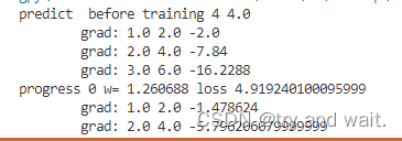

 

第一段代码是梯度下降，第二段代码是随机梯度下降

随机梯度下降法在神经网络中被证明是有效的。效率较低(时间复杂度较高)，学习性能较好。

随机梯度下降法和梯度下降法的主要区别在于：

1、损失函数由cost()更改为loss()。cost是计算所有训练数据的损失，loss是计算一个训练函数的损失。对应于源代码则是少了两个for循环。

2、梯度函数gradient()由计算所有训练数据的梯度更改为计算一个训练数据的梯度。

3、本算法中的随机梯度主要是指，每次拿一个训练数据来训练，然后更新梯度参数。本算法中梯度总共更新100(epoch)x3 = 300次。梯度下降法中梯度总共更新100(epoch)次。
————————————————
版权声明：本文为CSDN博主「错错莫」的原创文章，遵循CC 4.0 BY-SA版权协议，转载请附上原文出处链接及本声明。
原文链接：https://blog.csdn.net/bit452/article/details/109637108