深度学习训练营之优化器对比

最新推荐文章于 2024-05-27 13:58:30 发布

无你想你

最新推荐文章于 2024-05-27 13:58:30 发布

阅读量1.1k

点赞数

分类专栏：深度学习文章标签：深度学习 tensorflow 人工智能

本文链接：https://blog.csdn.net/qq_62904883/article/details/131126411

版权

深度学习专栏收录该内容

27 篇文章 1 订阅

订阅专栏

深度学习训练营之优化器对比

原文链接
环境介绍
前置工作
- 设置GPU
数据处理
模型构造
模型训练
结果可视化

原文链接

🍨 本文为🔗365天深度学习训练营中的学习记录博客
🍦 参考文章：365天深度学习训练营-第11周-优化器对比实验
🍖 原作者：K同学啊|接辅导、项目定制

环境介绍

语言环境：Python3.9.13
编译器：jupyter notebook
深度学习环境：TensorFlow2

前置工作

设置GPU

如果

import tensorflow as tf
gpus = tf.config.list_physical_devices("GPU")

if gpus:
    gpu0 = gpus[0] #如果有多个GPU，仅使用第0个GPU
    tf.config.experimental.set_memory_growth(gpu0, True) #设置GPU显存用量按需使用
    tf.config.set_visible_devices([gpu0],"GPU")

from tensorflow          import keras
import matplotlib.pyplot as plt
import pandas            as pd
import numpy             as np
import warnings,os,PIL,pathlib

warnings.filterwarnings("ignore")             #忽略警告信息
plt.rcParams['font.sans-serif']    = ['SimHei']  # 用来正常显示中文标签
plt.rcParams['axes.unicode_minus'] = False    # 用来正常显示负号

数据处理

导入数据

import pathlib

data_dir = "./29-data/"
data_dir = pathlib.Path(data_dir)
image_count = len(list(data_dir.glob('*/*')))
print("图片总数为：",image_count)

图片总数为： 1462

数据集处理

batch_size = 16#批量大小
img_height = 224
img_width  = 224
##在导入数据的过程当中打乱数据位置
train_ds=tf.keras.preprocessing.image_dataset_from_directory(
    data_dir,
    validation_split=0.2,
    subset="training",
    seed=24,#随机数种子
    image_size=(img_height,img_width),
    batch_size=batch_size
)

Found 1462 files belonging to 9 classes.
Using 1170 files for training.

##在导入数据的过程当中打乱数据位置
val_ds=tf.keras.preprocessing.image_dataset_from_directory(
    data_dir,
    validation_split=0.2,
    subset="validation",
    seed=24,#随机数种子
    image_size=(img_height,img_width),
    batch_size=batch_size
)

Found 1462 files belonging to 9 classes.
Using 292 files for validation.

class_names=train_ds.class_names
print("数据类型有:",class_names)
print("需要识别的船有%d类"%len(class_names))

数据类型有: [‘buoy’, ‘cruise ship’, ‘ferry boat’, ‘freight boat’, ‘gondola’, ‘inflatable boat’, ‘kayak’, ‘paper boat’, ‘sailboat’]
需要识别的船有9类

for image_batch,labels_batch in train_ds:
    print(image_batch.shape)
    print(labels_batch.shape)
    break

(16, 224, 224, 3)
(16,)

数据集可视化

AUTOTUNE = tf.data.AUTOTUNE

def train_preprocessing(image,label):
    return (image/255.0,label)

train_ds = (
    train_ds.cache()
    .map(train_preprocessing)    # 这里可以设置预处理函数
    .prefetch(buffer_size=AUTOTUNE)
)

val_ds = (
    val_ds.cache()
    .map(train_preprocessing)    # 这里可以设置预处理函数
    .prefetch(buffer_size=AUTOTUNE)
)

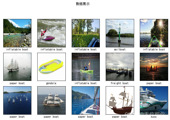
plt.figure(figsize=(10, 8))  # 图形的宽为10高为5
plt.suptitle("数据展示")

for images, labels in train_ds.take(1):
    for i in range(15):
        plt.subplot(4, 5, i + 1)
        plt.xticks([])
        plt.yticks([])
        plt.grid(False)

        # 显示图片
        plt.imshow(images[i])
        # 显示标签
        plt.xlabel(class_names[labels[i]-1])

plt.show()

请添加图片描述

模型构造

##对比不同优化器
from tensorflow.keras.layers import Dropout,Dense,BatchNormalization
from tensorflow.keras.models import Model

def create_model(optimizer='adam'):
    # 加载预训练模型
    vgg16_base_model = tf.keras.applications.vgg16.VGG16(weights='imagenet',
                                                                include_top=False,
                                                                input_shape=(img_width, img_height, 3),
                                                                pooling='avg')
    for layer in vgg16_base_model.layers:
        layer.trainable = False

    X = vgg16_base_model.output
    
    X = Dense(170, activation='relu')(X)
    X = BatchNormalization()(X)
    X = Dropout(0.5)(X)

    output = Dense(len(class_names), activation='softmax')(X)
    vgg16_model = Model(inputs=vgg16_base_model.input, outputs=output)

    vgg16_model.compile(optimizer=optimizer,
                        loss='sparse_categorical_crossentropy',
                        metrics=['accuracy'])
    return vgg16_model

model1 = create_model(optimizer=tf.keras.optimizers.Adam())
model2 = create_model(optimizer=tf.keras.optimizers.SGD())
model2.summary()

Downloading data from https://storage.googleapis.com/tensorflow/keras-applications/vgg16/vgg16_weights_tf_dim_ordering_tf_kernels_notop.h5
58889256/58889256 [==============================] - 60s 1us/step
Model: "model_1"
_________________________________________________________________
 Layer (type)                Output Shape              Param #   
=================================================================
 input_2 (InputLayer)        [(None, 224, 224, 3)]     0         
                                                                 
 block1_conv1 (Conv2D)       (None, 224, 224, 64)      1792      
                                                                 
 block1_conv2 (Conv2D)       (None, 224, 224, 64)      36928     
                                                                 
 block1_pool (MaxPooling2D)  (None, 112, 112, 64)      0         
                                                                 
 block2_conv1 (Conv2D)       (None, 112, 112, 128)     73856     
                                                                 
 block2_conv2 (Conv2D)       (None, 112, 112, 128)     147584    
                                                                 
 block2_pool (MaxPooling2D)  (None, 56, 56, 128)       0         
                                                                 
 block3_conv1 (Conv2D)       (None, 56, 56, 256)       295168    
                                                                 
 block3_conv2 (Conv2D)       (None, 56, 56, 256)       590080    
                                                                 
 block3_conv3 (Conv2D)       (None, 56, 56, 256)       590080    
...
Total params: 14,804,117
Trainable params: 89,089
Non-trainable params: 14,715,028
_________________________________________________________________
Output is truncated. View as a scrollable element or open in a text editor. Adjust cell output settings...

模型训练

开始进行模型训练

NO_EPOCHS = 50

history_model1  = model1.fit(train_ds, epochs=NO_EPOCHS, verbose=1, validation_data=val_ds)
history_model2  = model2.fit(train_ds, epochs=NO_EPOCHS, verbose=1, validation_data=val_ds)

Epoch 1/50
74/74 [==============================] - 82s 1s/step - loss: 1.6497 - accuracy: 0.4966 - val_loss: 1.4824 - val_accuracy: 0.6507
Epoch 2/50
74/74 [==============================] - 78s 1s/step - loss: 0.9829 - accuracy: 0.7043 - val_loss: 1.1832 - val_accuracy: 0.6952
Epoch 3/50
74/74 [==============================] - 78s 1s/step - loss: 0.8367 - accuracy: 0.7316 - val_loss: 0.9519 - val_accuracy: 0.7089
Epoch 4/50
74/74 [==============================] - 78s 1s/step - loss: 0.7420 - accuracy: 0.7684 - val_loss: 0.8481 - val_accuracy: 0.7021
Epoch 5/50
74/74 [==============================] - 79s 1s/step - loss: 0.6643 - accuracy: 0.7880 - val_loss: 0.8094 - val_accuracy: 0.7568
Epoch 6/50
74/74 [==============================] - 81s 1s/step - loss: 0.6044 - accuracy: 0.8060 - val_loss: 0.7265 - val_accuracy: 0.7705
Epoch 7/50
74/74 [==============================] - 81s 1s/step - loss: 0.5680 - accuracy: 0.8094 - val_loss: 0.7506 - val_accuracy: 0.7226
Epoch 8/50
74/74 [==============================] - 83s 1s/step - loss: 0.5108 - accuracy: 0.8333 - val_loss: 0.7361 - val_accuracy: 0.7534
Epoch 9/50
74/74 [==============================] - 84s 1s/step - loss: 0.4895 - accuracy: 0.8316 - val_loss: 0.8021 - val_accuracy: 0.7603
Epoch 10/50
74/74 [==============================] - 82s 1s/step - loss: 0.4669 - accuracy: 0.8470 - val_loss: 0.7546 - val_accuracy: 0.7568
Epoch 11/50
74/74 [==============================] - 82s 1s/step - loss: 0.4323 - accuracy: 0.8521 - val_loss: 0.8549 - val_accuracy: 0.7226
Epoch 12/50
74/74 [==============================] - 88s 1s/step - loss: 0.4015 - accuracy: 0.8778 - val_loss: 0.7263 - val_accuracy: 0.7671
Epoch 13/50
...
Epoch 49/50
74/74 [==============================] - 82s 1s/step - loss: 0.3593 - accuracy: 0.8880 - val_loss: 0.7675 - val_accuracy: 0.7808
Epoch 50/50
74/74 [==============================] - 81s 1s/step - loss: 0.3503 - accuracy: 0.8872 - val_loss: 0.7342 - val_accuracy: 0.7979
Output is truncated. View as a scrollable element or open in a text editor. Adjust cell output settings...

结果可视化

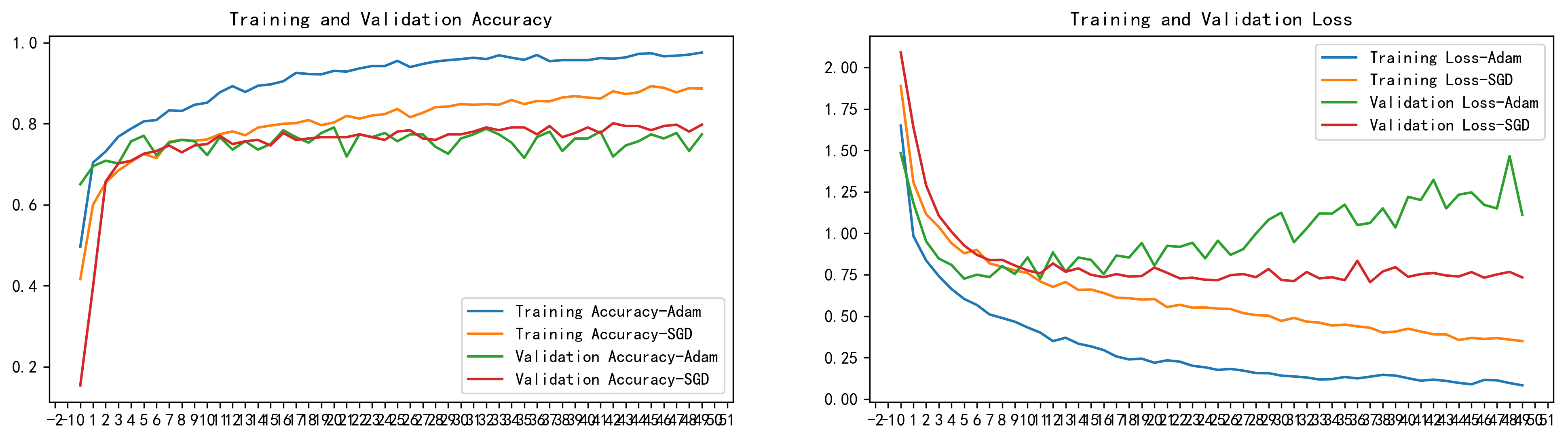
绘制两种不同训练方法的结果的图片

from matplotlib.ticker import MultipleLocator
plt.rcParams['savefig.dpi'] = 300 #图片像素
plt.rcParams['figure.dpi']  = 300 #分辨率

acc1     = history_model1.history['accuracy']
acc2     = history_model2.history['accuracy']
val_acc1 = history_model1.history['val_accuracy']
val_acc2 = history_model2.history['val_accuracy']

loss1     = history_model1.history['loss']
loss2     = history_model2.history['loss']
val_loss1 = history_model1.history['val_loss']
val_loss2 = history_model2.history['val_loss']

epochs_range = range(len(acc1))

plt.figure(figsize=(16, 4))
plt.subplot(1, 2, 1)

plt.plot(epochs_range, acc1, label='Training Accuracy-Adam')
plt.plot(epochs_range, acc2, label='Training Accuracy-SGD')
plt.plot(epochs_range, val_acc1, label='Validation Accuracy-Adam')
plt.plot(epochs_range, val_acc2, label='Validation Accuracy-SGD')
plt.legend(loc='lower right')
plt.title('Training and Validation Accuracy')
# 设置刻度间隔，x轴每1一个刻度
ax = plt.gca()
ax.xaxis.set_major_locator(MultipleLocator(1))

plt.subplot(1, 2, 2)
plt.plot(epochs_range, loss1, label='Training Loss-Adam')
plt.plot(epochs_range, loss2, label='Training Loss-SGD')
plt.plot(epochs_range, val_loss1, label='Validation Loss-Adam')
plt.plot(epochs_range, val_loss2, label='Validation Loss-SGD')
plt.legend(loc='upper right')
plt.title('Training and Validation Loss')
   
# 设置刻度间隔，x轴每1一个刻度
ax = plt.gca()
ax.xaxis.set_major_locator(MultipleLocator(1))

plt.show()

请添加图片描述

def test_accuracy_report(model):
    score = model.evaluate(val_ds, verbose=0)
    print('Loss function: %s, accuracy:' % score[0], score[1])
    
test_accuracy_report(model2)
test_accuracy_report(model1)