


 参数方程在数学中用于定义一组量作为独立变量(通常是时间)的函数。在动力学中,它们常用于表示物体的轨迹,通过时间参数化物体的位置、速度和加速度。在计算机辅助设计(CAD)中,参数方程有助于曲线和曲面的创建和操作。此外,在整数几何中,参数方程也用于解决特定问题,例如欧几里得的直角三角形参数化。参数方程可以是显式的,如直线和圆,也可以是隐式的,如椭圆和双曲线。在三维空间中,参数方程可以描述螺旋线和曲面,如螺线和高维流形。
In mathematics, a parametric equation defines a group of quantities as functions of one or more independent variables called parameters. Parametric equations are commonly used to express the coordinates of the points that make up a geometric object such as a curve or surface, in which case the equations are collectively called a parametric representation or parameterization (alternatively spelled as parametrisation) of the object.
For example, the equations
x
=
cos
t
y
=
sin
t
{\displaystyle {\begin{aligned}x&=\cos t\\y&=\sin t\end{aligned}}}
xy=cost=sint
form a parametric representation of the unit circle, where
t
t
t is the parameter: A point
(
x
,
y
)
(x, y)
(x,y) is on the unit circle if and only if there is a value of
t
t
t such that these two equations generate that point. Sometimes the parametric equations for the individual scalar output variables are combined into a single parametric equation in vectors:
(
x
,
y
)
=
(
cos
t
,
sin
t
)
.
{\displaystyle (x,y)=(\cos t,\sin t).}
(x,y)=(cost,sint).
Parametric representations are generally nonunique (see the “Examples in two dimensions” section below), so the same quantities may be expressed by a number of different parameterizations.
In addition to curves and surfaces, parametric equations can describe manifolds and algebraic varieties of higher dimension, with the number of parameters being equal to the dimension of the manifold or variety, and the number of equations being equal to the dimension of the space in which the manifold or variety is considered (for curves the dimension is one and one parameter is used, for surfaces dimension two and two parameters, etc.).
Parametric equations are commonly used in kinematics, where the trajectory of an object is represented by equations depending on time as the parameter. Because of this application, a single parameter is often labeled t t t; however, parameters can represent other physical quantities (such as geometric variables) or can be selected arbitrarily for convenience. Parameterizations are non-unique; more than one set of parametric equations can specify the same curve.
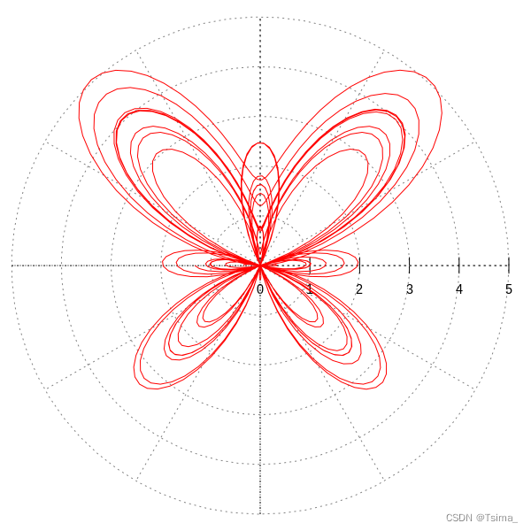
The butterfly curve can be defined by parametric equations of x x x and y y y.
Contents
1 Applications
1.1 Kinematics
In kinematics, objects’ paths through space are commonly described as parametric curves, with each spatial coordinate depending explicitly on an independent parameter (usually time). Used in this way, the set of parametric equations for the object’s coordinates collectively constitute a vector-valued function for position. Such parametric curves can then be integrated and differentiated termwise. Thus, if a particle’s position is described parametrically as
r
(
t
)
=
(
x
(
t
)
,
y
(
t
)
,
z
(
t
)
)
{\displaystyle \mathbf {r} (t)=(x(t),y(t),z(t))}
r(t)=(x(t),y(t),z(t))
then its velocity can be found as
v
(
t
)
=
r
′
(
t
)
=
(
x
′
(
t
)
,
y
′
(
t
)
,
z
′
(
t
)
)
{\displaystyle \mathbf {v} (t)=\mathbf {r} '(t)=(x'(t),y'(t),z'(t))}
v(t)=r′(t)=(x′(t),y′(t),z′(t))
and its acceleration as
a
(
t
)
=
r
′
′
(
t
)
=
(
x
′
′
(
t
)
,
y
′
′
(
t
)
,
z
′
′
(
t
)
)
{\displaystyle \mathbf {a} (t)=\mathbf {r} ''(t)=(x''(t),y''(t),z''(t))}
a(t)=r′′(t)=(x′′(t),y′′(t),z′′(t))
1.2 Computer-aided design
Another important use of parametric equations is in the field of computer-aided design (CAD). For example, consider the following three representations, all of which are commonly used to describe planar curves.
| Type | Form | Example | Description |
|---|---|---|---|
| Explicit | y = f ( x ) {\displaystyle y=f(x)\,\!} y=f(x) | y = m x + b {\displaystyle y=mx+b\,\!} y=mx+b | Line |
| Implicit | f ( x , y ) = 0 {\displaystyle f(x,y)=0\,\!} f(x,y)=0 | ( x − a ) 2 + ( y − b ) 2 = r 2 {\displaystyle \left(x-a\right)^{2}+\left(y-b\right)^{2}=r^{2}} (x−a)2+(y−b)2=r2 | Circle |
| Parametric | x = g ( t ) w ( t ) ; y = h ( t ) w ( t ) {\displaystyle x={\frac {g(t)}{w(t)}};\,\!} \ {\displaystyle y={\frac {h(t)}{w(t)}}} x=w(t)g(t); y=w(t)h(t) | x = a 0 + a 1 t ; y = b 0 + b 1 t {\displaystyle x=a_{0}+a_{1}t;\,\!} \ {\displaystyle y=b_{0}+b_{1}t\,\!} x=a0+a1t; y=b0+b1t | Line |
| Parametric | x = g ( t ) w ( t ) ; y = h ( t ) w ( t ) {\displaystyle x={\frac {g(t)}{w(t)}};\,\!} \ {\displaystyle y={\frac {h(t)}{w(t)}}} x=w(t)g(t); y=w(t)h(t) | x = a + r cos t ; y = b + r sin t {\displaystyle x=a+r\,\cos t;\,\!}\ {\displaystyle y=b+r\,\sin t\,\!} x=a+rcost; y=b+rsint | Circle |
Each representation has advantages and drawbacks for CAD applications.
The explicit representation may be very complicated, or even may not exist. Moreover, it does not behave well under geometric transformations, and in particular under rotations. On the other hand, as a parametric equation and an implicit equation may easily be deduced from an explicit representation, when a simple explicit representation exists, it has the advantages of both other representations.
Implicit representations may make it difficult to generate points on the curve, and even to decide whether there are real points. On the other hand, they are well suited for deciding whether a given point is on a curve, or whether it is inside or outside of a closed curve.
Such decisions may be difficult with a parametric representation, but parametric representations are best suited for generating points on a curve, and for plotting it.
1.3 Integer geometry
Numerous problems in integer geometry can be solved using parametric equations. A classical such solution is Euclid’s parametrization of right triangles such that the lengths of their sides
a
,
b
a, b
a,b and their hypotenuse
c
c
c are coprime integers. As
a
a
a and
b
b
b are not both even (otherwise
a
,
b
a, b
a,b and
c
c
c would not be coprime), one may exchange them to have
a
a
a even, and the parameterization is then
a
=
2
m
n
,
b
=
m
2
−
n
2
,
c
=
m
2
+
n
2
,
{\displaystyle a=2mn,\ \ b=m^{2}-n^{2},\ \ c=m^{2}+n^{2},}
a=2mn, b=m2−n2, c=m2+n2,
where the parameters
m
m
m and
n
n
n are positive coprime integers that are not both odd.
By multiplying a , b a, b a,b and c c c by an arbitrary positive integer, one gets a parametrization of all right triangles whose three sides have integer lengths.
2 Implicitization
Converting a set of parametric equations to a single implicit equation involves eliminating the variable t {\displaystyle t} t from the simultaneous equations x = f ( t ) , y = g ( t ) . {\displaystyle x=f(t),\ y=g(t).} x=f(t), y=g(t). This process is called implicitization. If one of these equations can be solved for t t t, the expression obtained can be substituted into the other equation to obtain an equation involving x x x and y y y only: Solving y = g ( t ) {\displaystyle y=g(t)} y=g(t) to obtain t = g − 1 ( y ) {\displaystyle t=g^{-1}(y)} t=g−1(y) and using this in x = f ( t ) {\displaystyle x=f(t)} x=f(t) gives the explicit equation x = f ( g − 1 ( y ) ) , {\displaystyle x=f(g^{-1}(y)),} x=f(g−1(y)), while more complicated cases will give an implicit equation of the form h ( x , y ) = 0. {\displaystyle h(x,y)=0.} h(x,y)=0.
If the parametrization is given by rational functions
x
=
p
(
t
)
r
(
t
)
,
y
=
q
(
t
)
r
(
t
)
,
{\displaystyle x={\frac {p(t)}{r(t)}},\qquad y={\frac {q(t)}{r(t)}},}
x=r(t)p(t),y=r(t)q(t),
where
p
,
q
,
r
p, q, r
p,q,r are set-wise coprime polynomials, a resultant computation allows one to implicitize. More precisely, the implicit equation is the resultant with respect to
t
t
t of
x
r
(
t
)
–
p
(
t
)
xr(t) – p(t)
xr(t)–p(t) and
y
r
(
t
)
–
q
(
t
)
yr(t) – q(t)
yr(t)–q(t)
In higher dimensions (either more than two coordinates or more than one parameter), the implicitization of rational parametric equations may by done with Gröbner basis computation; see Gröbner basis § Implicitization in higher dimension.
To take the example of the circle of radius
a
a
a, the parametric equations
x
=
a
cos
(
t
)
y
=
a
sin
(
t
)
{\displaystyle {\begin{aligned}x&=a\cos(t)\\y&=a\sin(t)\end{aligned}}}
xy=acos(t)=asin(t)
can be implicitized in terms of
x
x
x and
y
y
y by way of the Pythagorean trigonometric identity:
As
x
a
=
cos
(
t
)
y
a
=
sin
(
t
)
{\displaystyle {\begin{aligned}{\frac {x}{a}}&=\cos(t)\\{\frac {y}{a}}&=\sin(t)\\\end{aligned}}}
axay=cos(t)=sin(t)
and
cos
(
t
)
2
+
sin
(
t
)
2
=
1
,
{\displaystyle \cos(t)^{2}+\sin(t)^{2}=1,}
cos(t)2+sin(t)2=1,
we get
(
x
a
)
2
+
(
y
a
)
2
=
1
,
{\displaystyle \left({\frac {x}{a}}\right)^{2}+\left({\frac {y}{a}}\right)^{2}=1,}
(ax)2+(ay)2=1,
and thus
x
2
+
y
2
=
a
2
,
{\displaystyle x^{2}+y^{2}=a^{2},}
x2+y2=a2,
which is the standard equation of a circle centered at the origin.
3 Examples in two dimensions
3.1 Parabola
The simplest equation for a parabola,
y
=
x
2
{\displaystyle y=x^{2}\,}
y=x2
can be (trivially) parameterized by using a free parameter
t
t
t, and setting
x
=
t
,
y
=
t
2
f
o
r
−
∞
<
t
<
∞
.
{\displaystyle x=t,y=t^{2}\quad \mathrm {for} -\infty <t<\infty .\,}
x=t,y=t2for−∞<t<∞.
3.2 Explicit equations
More generally, any curve given by an explicit equation
y
=
f
(
x
)
{\displaystyle y=f(x)\,}
y=f(x)
can be (trivially) parameterized by using a free parameter t, and setting
x
=
t
,
y
=
f
(
t
)
f
o
r
−
∞
<
t
<
∞
.
{\displaystyle x=t,y=f(t)\quad \mathrm {for} -\infty <t<\infty .\,}
x=t,y=f(t)for−∞<t<∞.
3.3 Circle
A more sophisticated example is the following. Consider the unit circle which is described by the ordinary (Cartesian) equation
x
2
+
y
2
=
1.
{\displaystyle x^{2}+y^{2}=1.\,}
x2+y2=1.
This equation can be parameterized as follows:
(
x
,
y
)
=
(
cos
(
t
)
,
sin
(
t
)
)
f
o
r
0
≤
t
<
2
π
.
{\displaystyle (x,y)=(\cos(t),\;\sin(t))\quad \mathrm {for} \ 0\leq t<2\pi .\,}
(x,y)=(cos(t),sin(t))for 0≤t<2π.
With the Cartesian equation it is easier to check whether a point lies on the circle or not. With the parametric version it is easier to obtain points on a plot.
In some contexts, parametric equations involving only rational functions (that is fractions of two polynomials) are preferred, if they exist. In the case of the circle, such a rational parameterization is
x
=
1
−
t
2
1
+
t
2
y
=
2
t
1
+
t
2
.
{\displaystyle {\begin{aligned}x&={\frac {1-t^{2}}{1+t^{2}}}\\y&={\frac {2t}{1+t^{2}}}\end{aligned}}.}
xy=1+t21−t2=1+t22t.
With this pair of parametric equations, the point
(
−
1
,
0
)
(−1, 0)
(−1,0) is not represented by a real value of
t
t
t, but by the limit of
x
x
x and
y
y
y when
t
t
t tends to infinity.
3.4 Ellipse
An ellipse in canonical position (center at origin, major axis along the
X
X
X-axis) with semi-axes
a
a
a and
b
b
b can be represented parametrically as
x
=
a
cos
t
y
=
b
sin
t
.
{\displaystyle {\begin{aligned}x&=a\,\cos t\\y&=b\,\sin t.\end{aligned}}}
xy=acost=bsint.
An ellipse in general position can be expressed as
x
=
X
c
+
a
cos
t
cos
φ
−
b
sin
t
sin
φ
y
=
Y
c
+
a
cos
t
sin
φ
+
b
sin
t
cos
φ
{\displaystyle {\begin{aligned}x&=X_{c}+a\,\cos t\,\cos \varphi -b\,\sin t\,\sin \varphi \\y&=Y_{c}+a\,\cos t\,\sin \varphi +b\,\sin t\,\cos \varphi \end{aligned}}}
xy=Xc+acostcosφ−bsintsinφ=Yc+acostsinφ+bsintcosφ
as the parameter
t
t
t varies from
0
0
0 to
2
π
2π
2π. Here
(
X
c
,
Y
c
)
{\displaystyle (X_{c},Y_{c})}
(Xc,Yc) is the center of the ellipse, and
φ
{\displaystyle \varphi }
φ is the angle between the
X
{\displaystyle X}
X-axis and the major axis of the ellipse.
Both parameterizations may be made rational by using the tangent half-angle formula and setting tan t 2 = u . {\displaystyle \tan {\frac {t}{2}}=u.} tan2t=u.
3.5 Lissajous Curve
A Lissajous curve is similar to an ellipse, but the
x
x
x and
y
y
y sinusoids are not in phase. In canonical position, a Lissajous curve is given by
x
=
a
cos
(
k
x
t
)
y
=
b
sin
(
k
y
t
)
{\displaystyle {\begin{aligned}x&=a\,\cos(k_{x}t)\\y&=b\,\sin(k_{y}t)\end{aligned}}}
xy=acos(kxt)=bsin(kyt)
where
k
x
{\displaystyle k_{x}}
kx and
k
y
{\displaystyle k_{y}}
ky are constants describing the number of lobes of the figure.
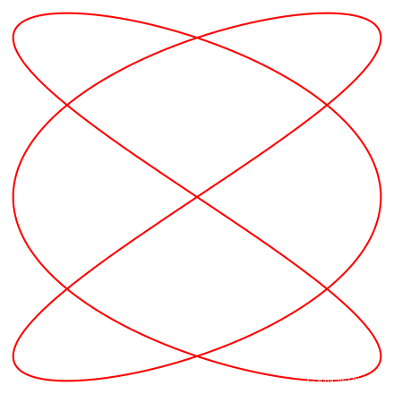
A Lissajous curve where k x = 3 {\displaystyle k_{x}=3} kx=3 and k y = 2 {\displaystyle k_{y}=2} ky=2.
3.6 Hyperbola
An east-west opening hyperbola can be represented parametrically by
x
=
a
sec
t
+
h
y
=
b
tan
t
+
k
{\displaystyle {\begin{aligned}x&=a\sec t+h\\y&=b\tan t+k\end{aligned}}\quad }
xy=asect+h=btant+k
or, rationally
x
=
a
1
+
t
2
1
−
t
2
+
h
y
=
b
2
t
1
−
t
2
+
k
{\displaystyle \quad {\begin{aligned}x&=a{\frac {1+t^{2}}{1-t^{2}}}+h\\y&=b{\frac {2t}{1-t^{2}}}+k\end{aligned}}}
xy=a1−t21+t2+h=b1−t22t+k
A north-south opening hyperbola can be represented parametrically as
x
=
b
tan
t
+
h
y
=
a
sec
t
+
k
{\displaystyle {\begin{matrix}x=b\tan t+h\\y=a\sec t+k\\\end{matrix}}\quad }
x=btant+hy=asect+k
or, rationally
x
=
b
2
t
1
−
t
2
+
h
y
=
a
1
+
t
2
1
−
t
2
+
k
{\displaystyle \quad {\begin{matrix}x=b{\frac {2t}{1-t^{2}}}+h\\y=a{\frac {1+t^{2}}{1-t^{2}}}+k\\\end{matrix}}}
x=b1−t22t+hy=a1−t21+t2+k
In all these formulae ( h , k ) (h, k) (h, k) are the center coordinates of the hyperbola, a a a is the length of the semi-major axis, and b b b is the length of the semi-minor axis.
3.7 Hypotrochoid
A hypotrochoid is a curve traced by a point attached to a circle of radius r r r rolling around the inside of a fixed circle of radius R R R, where the point is at a distance d d d from the center of the interior circle.
The parametric equations for the hypotrochoids are:
x
(
θ
)
=
(
R
−
r
)
cos
θ
+
d
cos
(
R
−
r
r
θ
)
y
(
θ
)
=
(
R
−
r
)
sin
θ
−
d
sin
(
R
−
r
r
θ
)
{\displaystyle {\begin{aligned}x(\theta )&=(R-r)\cos \theta +d\cos \left({R-r \over r}\theta \right)\\y(\theta )&=(R-r)\sin \theta -d\sin \left({R-r \over r}\theta \right)\end{aligned}}}
x(θ)y(θ)=(R−r)cosθ+dcos(rR−rθ)=(R−r)sinθ−dsin(rR−rθ)
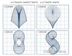
3.8 Some sophisticated functions
Other examples are shown:
x
=
[
a
−
b
]
cos
(
t
)
+
b
cos
[
t
(
a
b
−
1
)
]
y
=
[
a
−
b
]
sin
(
t
)
−
b
sin
[
t
(
a
b
−
1
)
]
,
k
=
a
b
{\displaystyle {\begin{aligned}x&=[a-b]\cos(t)\ +b\cos \left[t\left({\frac {a}{b}}-1\right)\right]\\y&=[a-b]\sin(t)\ -b\sin \left[t\left({\frac {a}{b}}-1\right)\right],\ k={\frac {a}{b}}\end{aligned}}}
xy=[a−b]cos(t) +bcos[t(ba−1)]=[a−b]sin(t) −bsin[t(ba−1)], k=ba
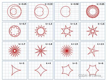
Several graphs by variation of k k k
x
=
cos
(
a
t
)
−
cos
(
b
t
)
j
y
=
sin
(
c
t
)
−
sin
(
d
t
)
k
{\begin{aligned}x&=\cos(at)-\cos(bt)^{j}\\y&=\sin(ct)-\sin(dt)^{k}\end{aligned}}
xy=cos(at)−cos(bt)j=sin(ct)−sin(dt)k
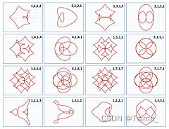
x
=
i
cos
(
a
t
)
−
cos
(
b
t
)
sin
(
c
t
)
y
=
j
sin
(
d
t
)
−
sin
(
e
t
)
{\begin{aligned}x&=i\cos(at)-\cos(bt)\sin(ct)\\y&=j\sin(dt)-\sin(et)\end{aligned}}
xy=icos(at)−cos(bt)sin(ct)=jsin(dt)−sin(et)
4 Examples in three dimensions
4.1 Helix
Parametric equations are convenient for describing curves in higher-dimensional spaces. For example:
x
=
a
cos
(
t
)
y
=
a
sin
(
t
)
z
=
b
t
{\displaystyle {\begin{aligned}x&=a\cos(t)\\y&=a\sin(t)\\z&=bt\,\end{aligned}}}
xyz=acos(t)=asin(t)=bt
describes a three-dimensional curve, the helix, with a radius of
a
a
a and rising by
2
π
b
2πb
2πb units per turn. The equations are identical in the plane to those for a circle. Such expressions as the one above are commonly written as
r
(
t
)
=
(
x
(
t
)
,
y
(
t
)
,
z
(
t
)
)
=
(
a
cos
(
t
)
,
a
sin
(
t
)
,
b
t
)
,
{\displaystyle \mathbf {r} (t)=(x(t),y(t),z(t))=(a\cos(t),a\sin(t),bt),}
r(t)=(x(t),y(t),z(t))=(acos(t),asin(t),bt),
where
r
r
r is a three-dimensional vector.
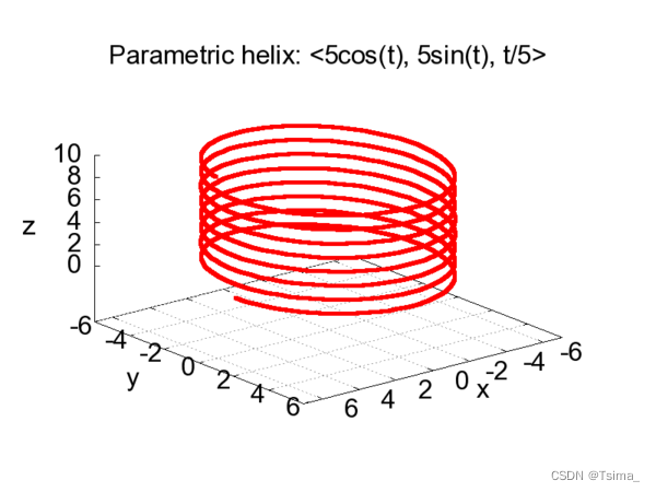
Parametric helix
4.2 Parametric surfaces
Main article: Parametric surface
A torus with major radius
R
R
R and minor radius
r
r
r may be defined parametrically as
x
=
cos
(
t
)
(
R
+
r
cos
(
u
)
)
,
y
=
sin
(
t
)
(
R
+
r
cos
(
u
)
)
,
z
=
r
sin
(
u
)
.
{\displaystyle {\begin{aligned}x&=\cos(t)\left(R+r\cos(u)\right),\\y&=\sin(t)\left(R+r\cos(u)\right),\\z&=r\sin(u).\end{aligned}}}
xyz=cos(t)(R+rcos(u)),=sin(t)(R+rcos(u)),=rsin(u).
where the two parameters
t
t
t and
u
u
u both vary between
0
0
0 and
2
π
2π
2π.
As u u u varies from 0 0 0 to 2 π 2π 2π the point on the surface moves about a short circle passing through the hole in the torus. As t t t varies from 0 0 0 to 2 π 2π 2π the point on the surface moves about a long circle around the hole in the torus.
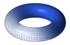
R = 2 , r = 1 / 2 R = 2, r = 1/2 R=2,r= 1/2
5 Examples with vectors
The parametric equation of the line through the point
(
x
0
,
y
0
,
z
0
)
{\displaystyle \left(x_{0},y_{0},z_{0}\right)}
(x0,y0,z0) and parallel to the vector
a
i
^
+
b
j
^
+
c
k
^
{\displaystyle a{\hat {\mathbf {i} }}+b{\hat {\mathbf {j} }}+c{\hat {\mathbf {k} }}}
ai^+bj^+ck^ is
x
=
x
0
+
a
t
y
=
y
0
+
b
t
z
=
z
0
+
c
t
{\displaystyle {\begin{aligned}x&=x_{0}+at\\y&=y_{0}+bt\\z&=z_{0}+ct\end{aligned}}}
xyz=x0+at=y0+bt=z0+ct
6 See also
- Curve
- Parametric estimating
- Position vector
- Vector-valued function
- Parametrization by arc length
- Parametric derivative
7 Notes
@Skip
8 External links
@Skip


 4034
4034

 被折叠的 条评论
为什么被折叠?
被折叠的 条评论
为什么被折叠?
 到【灌水乐园】发言


