Farrow任意采样率变换matlab仿真

Farrow结构是用于任意采样率变换的一种有效方法。它通过使用多项式插值技术实现对离散时间信号进行采样率变换，适用于多种通信系统和信号处理应用。以下是Farrow任意采样率变换的原理及其关键要点：

1. 基本原理
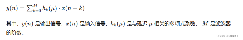
   Farrow结构基于多项式插值，用于实现任意采样率变换。具体来说，它使用由Farrow提出的多项式滤波器结构，通过线性组合不同延迟的信号样本实现插值。其主要优势在于它能够动态调整采样率，而无需重新设计滤波器。

2. 多项式插值
   多项式插值的基本思想是使用多项式函数来估计未知采样点的值。Farrow结构通常使用Lagrange插值多项式或FIR滤波器实现这一点。Lagrange插值多项式可以精确地通过给定的样本点，从而提供高精度的插值结果。

3. Farrow结构
   Farrow结构可以表示为一组并行的FIR滤波器，每个滤波器具有不同的系数。这些系数由输入信号的延迟量决定。Farrow结构的典型形式包括：
   

4. 多项式系数的计算
   Farrow结构中的多项式系数通常通过预先计算并存储在查找表中，以便在运行时快速查找。这些系数可以根据不同的插值阶数和采样率变化范围进行调整。

5. 动态采样率变换
   Farrow结构的一个重要特点是其动态采样率变换能力。通过调整插值多项式的系数，可以实现任意的采样率变换。这使得Farrow结构在需要频繁改变采样率的应用中非常有效，例如在软件无线电和多速率信号处理系统中。

% **************************************************************
% Vectorized Farrow resampler
% M. Nentwig, 2011
% Note: Uses cyclic signals (wraps around)
% **************************************************************
close all; clear all;
 
% inData contains input to the resampling process (instead of function arguments)
inData = struct();
%%  farrow rate change factor
% if rational, use format R=P/Q=f_out/f_in
% P = 10;
% Q = 9;
%% 设置成型滤波器
M = 15;
L = 14;
Len = M*L+1;
sps = 5;
span = (Len-1)/sps;
beta = 0.22;
Len = sps * span + 1;
%[h_Rs_coe Len]= generate_RS_coe(span,sps,beta);
%h_Rs_coe = h_Rs_coe./max(h_Rs_coe);
%% 拟合成型滤波器的系数
% L = 14;
K = 3;
%[P e] = construct_farrow(h_Rs_coe,L,K);

% **************************************************************
% example coefficients. 
% Each column [c0; c1; c2; c3] describes a polynomial for one tap coefficent in fractional time ft [0, 1]:
% tapCoeff = c0 + c1 * ft + c2 * ft ^ 2 + c3 * ft ^ 3
% Each column corresponds to one tap. 
% the matrix size may be changed arbitrarily.
% 
% The example filter is based on a 6th order Chebyshev Laplace-domain prototype.
% **************************************************************
% inData.cMatrix =[ -8.57738278e-3 7.82989032e-1 7.19303539e+000 6.90955718e+000 -2.62377450e+000 -6.85327127e-1 1.44681608e+000 -8.79147907e-1 7.82633997e-2 1.91318985e-1 -1.88573400e-1 6.91790782e-2 3.07723786e-3 -6.74800912e-3
%  2.32448021e-1 2.52624309e+000 7.67543936e+000 -8.83951796e+000 -5.49838636e+000 6.07298348e+000 -2.16053205e+000 -7.59142947e-1 1.41269409e+000 -8.17735712e-1 1.98119464e-1 9.15904145e-2 -9.18092030e-2 2.74136108e-2
%  -1.14183319e+000 6.86126458e+000 -6.86015957e+000 -6.35135894e+000 1.10745051e+001 -3.34847578e+000 -2.22405694e+000 3.14374725e+000 -1.68249886e+000 2.54083065e-1 3.22275037e-1 -3.04794927e-1 1.29393976e-1 -3.32026332e-2
%  1.67363115e+000 -2.93090391e+000 -1.13549165e+000 5.65274939e+000 -3.60291782e+000 -6.20715544e-1 2.06619782e+000 -1.42159644e+000 3.75075865e-1 1.88433333e-1 -2.64135123e-1 1.47117661e-1 -4.71871047e-2 1.24921920e-2
% ] / 12.28;
% A =[0 0 1.0000 0 -0.0165 0.1045 0.9405 -0.0285 -0.0320 0.2160 0.8640 -0.0480 -0.0455 0.3315 0.7735 -0.0595 -0.0560 0.4480 0.6720 -0.0640 -0.0625 0.5625 0.5625 -0.0625 -0.0640 0.6720 0.4480 -0.0560 -0.0595 0.7735 0.3315 -0.0455 -0.0480 0.8640 0.2160 -0.0320 -0.0285 0.9405 0.1045 -0.0165];
% B = reshape(A.',4,[]);

inData.cMatrix =[ -8.57738278e-3 7.82989032e-1 7.19303539e+000 6.90955718e+000 -2.62377450e+000 -6.85327127e-1 1.44681608e+000 -8.79147907e-1 7.82633997e-2 1.91318985e-1 -1.88573400e-1 6.91790782e-2 3.07723786e-3 -6.74800912e-3
 2.32448021e-1 2.52624309e+000 7.67543936e+000 -8.83951796e+000 -5.49838636e+000 6.07298348e+000 -2.16053205e+000 -7.59142947e-1 1.41269409e+000 -8.17735712e-1 1.98119464e-1 9.15904145e-2 -9.18092030e-2 2.74136108e-2
 -1.14183319e+000 6.86126458e+000 -6.86015957e+000 -6.35135894e+000 1.10745051e+001 -3.34847578e+000 -2.22405694e+000 3.14374725e+000 -1.68249886e+000 2.54083065e-1 3.22275037e-1 -3.04794927e-1 1.29393976e-1 -3.32026332e-2
 1.67363115e+000 -2.93090391e+000 -1.13549165e+000 5.65274939e+000 -3.60291782e+000 -6.20715544e-1 2.06619782e+000 -1.42159644e+000 3.75075865e-1 1.88433333e-1 -2.64135123e-1 1.47117661e-1 -4.71871047e-2 1.24921920e-2
];
% inData.cMatrix  = P;
% inData.cMatrix =[   0.95142 	-0.097163 	-0.048581; 
%                     0.56277 	-0.29149 	-0.048581; 
%                     -0.10323 	-0.21284	0.11309; 
%                     -0.17114    0.050361	0.018514; 
%                     -0.016682	0.08377 	-0.0018097; 
%                     0.10629     0.0018814 	-0.039135];
% inData.cMatrix = [0.0890316291775468,0.382074655730815,-0.541134925405564,0.0546010437714621;-1.41066423272581,1.75403675048886,0.650677747278054,0.00391231449097261;1.41066423272581,-2.47795594768857,0.0732414499216628,0.997962579532074;-0.0890316291775541,0.649169543263466,-0.490109273588710,-0.0154275967257404];

         
P_SUM = sum(sum(inData.cMatrix));
inData.cMatrix =inData.cMatrix./P_SUM;
% inData.cMatrix = P;
 pp = reshape(inData.cMatrix,[],1);
 fvtool(pp)
% **************************************************************
% Create example signal
% **************************************************************
nIn = 50; % used for test signal generation only
if true
    % complex signal
    inData.signal = cos(2*pi*(0:(nIn-1)) / nIn);% + cos(2*2*pi*(0:(nIn-1)) / nIn) + 1.5;
else
    % impulse response
    inData.signal = zeros(1, nIn); inData.signal(1) = 1; % 
 
    % inData.cMatrix = 0 * inData.cMatrix; inData.cMatrix(1, 1) = 1; % enable to show constant c in first tap
    % inData.cMatrix = 0 * inData.cMatrix; inData.cMatrix(2, 1) = 1; % enable to show linear c in first tap
    % inData.cMatrix = 0 * inData.cMatrix; inData.cMatrix(3, 1) = 1; % enable to show quadratic c in first tap
    % inData.cMatrix = 0 * inData.cMatrix; inData.cMatrix(1, 2) = 1; % enable to show constant c in second tap
end
 
% **************************************************************
% Resample to the following number of output samples
% must be integer, otherwise arbitrary
% **************************************************************
fs1 = 23e6;
fs2 = 12e6;
K = fs2/fs1;
inData.nSamplesOut = floor(nIn * K);
 
% **************************************************************
% Set up Farrow resampling
% **************************************************************
nSamplesIn = size(inData.signal, 2);
nSamplesOut = inData.nSamplesOut;
order = size(inData.cMatrix, 1) - 1; % polynomial order
nTaps = size(inData.cMatrix, 2); % number of input samples that contribute to one output sample (FIR size)
 
% pointer to the position in the input stream for each output sample (row vector, real numbers), starting at 0
inputIndex = (0:nSamplesOut-1) / nSamplesOut * nSamplesIn;
 
% split into integer part (0..nSamplesIn - 1) ...
inputIndexIntegerPart = floor(inputIndex);
% ... and fractional part [0, 1[
inputIndexFractionalPart = inputIndex - inputIndexIntegerPart;
 
% **************************************************************
% Calculate output stream
% First constant term (conventional FIR), then linear, quadratic, cubic, ... 
% **************************************************************
outStream = zeros(1, inData.nSamplesOut);
for ixOrder = 0 : order
    x = inputIndexFractionalPart .^ ixOrder;
    
    % **************************************************************
    % Add the contribution of each tap one-by-one
    % **************************************************************
    for ixTap = 0 : nTaps - 1
        c = inData.cMatrix(ixOrder+1, ixTap+1);
        % index of input sample that contributes to output via the current tap
        % higher tap index => longer delay => older input sample => smaller data index
        dataIx = inputIndexIntegerPart - ixTap;
        % wrap around
        dataIx = mod(dataIx, nSamplesIn);
        % array indexing starts at 1
        dataIx = dataIx + 1;
        delayed = inData.signal(dataIx);
        % for each individual output sample (index in row vector), 
        % - evaluate f = c(order, tapindex) * fracPart .^ order 
        % - scale the delayed input sample with f
        % - accumulate the contribution of all taps
        % this implementation performs the operation for all output samples in parallel (row vector)
        outStream = outStream + c * delayed .* x;
    end % for ixTap
end % for ixOrder
 
% **************************************************************
% plot
% **************************************************************
xIn = linspace(0, 1, nSamplesIn + 1); xIn = xIn(1:end-1);
xOut = linspace(0, 1, nSamplesOut + 1); xOut = xOut(1:end-1);
 
figure(); grid on; hold on;
stem(xIn, inData.signal, 'k+-');
plot(xOut, outStream(), 'b+-');
legend('input', 'output');
title('Farrow resampling. Signals are cyclic');