图像处理（一）基于特征的图像对齐算法

一、介绍

1.1 图像对齐是什么？

图像对齐(或者图像配准)可以扭曲旋转（其实是仿射变换）一张图使它和另一个图可以很完美的对齐。
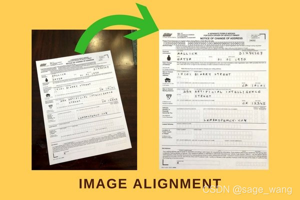
下面是一个例子，中间的表在经过图像对齐技术处理之后，可以和左边的模板一样。对齐之后就可以根据模板的格式对用户填写的内容进行分析了。

1.2 图像对齐算法的应用场景有哪些？

图像对齐技术广泛应用于计算机视觉各类任务

• 对不同视角下拍摄的图片进行拼接（Image stitching）
• 智能手机等摄像设备在Burst模式下的图像降噪
• 图像超分辨率应用
• 视频防抖
• 生成基于多次曝光的高动态范围HDR图像
• 医学图像领域
• 跨模态数据的对齐任务

1.3 图像对齐算法有哪些？

图像对齐的传统方法而言，总体上可以分为三大类：

• Homography： 对应为3x3变换矩阵。（本文主要介绍这个方法）
• MeshFlow：是一个空间光滑的稀疏运动场，运动矢量位于网格顶点。
• Optical flow（光流）法：光流法是利用图像序列中像素在时间域上的变化以及相邻帧之间的相关性来找到上一帧跟当前帧之间存在的对应关系，从而计算出相邻帧之间物体的运动信息的一种方法。

1.4 Homopgraphy是什么？

要想使用单应性矩阵把同一个场景的两张照片联系起来，需要两个条件：

• 两张照片中拍摄了同一个平面
• 这两幅照片是通过旋转照相机的光学轴来拍摄的。我们在生成全景图的同时就是这么做的。

单应性矩阵就是一个简单的3X3的矩阵：

所谓Homography变换，中文称之为透视变换，对应为3x3变换矩阵称之为单应性矩阵，如下图H。
$$\left[\begin{array}{ccc}h00& h01& h02\\ h10& h11& h12\\ h20& h21& h22\end{array}\right]\text{\hspace{1em}(3)}$$

假设(x1,y1)是第一张图片上的点，(x2,y2)是第二张图片上的同一个物理点，那么使用单应性矩阵可以映射他们：

1.5 ORB是什么？

ORB的本质是带方向的FAST特征点和旋转的BRIEF描述子 的 特征点检测器。

一个特征点检测器由两部分组成：

1.定位器：这个模块要找到图片上具有旋转不变性、缩放不变性及仿射不变性的点。定位器找到这些点的x/y坐标。ORB的定位器被称为FAST。这种寻找特征点的算法一听就知道，很快嘛。

2.描述子：上一步只是找到特征点在哪，这一步要获得它们的外观编码来区分彼此。这样特征点就可以使用被称为描述子的一串数字来表示了。理想情况下，不同照片上对应的同一个物理点应该具有相同的描述子。ORB的描述子是一种改进的BRISK描述子.

由于只有知道两张图片特征点对应关系的情况下才能计算两图的单应性矩阵，所以我们需要一个算法来自动匹配两图的特征点。这个算法将会把两图的特征点一一比较。

二、Demo展示

opencv图像对齐 ，基于特征的图像对齐步骤，下面的代码进行图像对齐的步骤

• 读取图片到内存。
• 检测特征点：为两张图检测ORB特征点。为了计算单应性矩阵4个就够了，但是一般会检测到成百上千的特征点。可以使用参数MAX_FEATURES 来控制检测的特征点的数量。检测特征点并计算描述子的函数是detectAndCompute。
• 特征匹配：找到两图中匹配的特征点，并按照匹配度排列，保留最匹配的一小部分。然后把匹配的特征点画出来并保存图片到磁盘。我们使用汉明距离来度量两个特征点描述子的相似度。下图中把匹配的特征点用线连起来了。注意，有很多错误匹配的特征点，所以下一步要用一个健壮的算法来计算单应性矩阵。
• 计算单应性矩阵：上一步产生的匹配的特征点不是100%正确的，就算只有20~30%的匹配是正确的也不罕见。findHomography 函数使用一种被称为随机抽样一致算法(Random Sample Consensus )的技术在大量匹配错误的情况下计算单应性矩阵。
• 扭转图片(Warping image)：有了精确的单应性矩阵，就可以把一张图片的所有像素映射到另一个图片。warpPerspective 函数用来完成这个功能。

bighead_cat.jpg （网红大头喵镇楼）

bighead_cat_45.jpg 旋转45度后的图片，作为需要对齐的图片。

from __future__ import print_function
import cv2
import numpy as np


MAX_FEATURES = 500
GOOD_MATCH_PERCENT = 0.15



def drawMatches(img1, kp1, img2, kp2, matches):
    """
    My own implementation of cv2.drawMatches as OpenCV 2.4.9
    does not have this function available but it's supported in
    OpenCV 3.0.0

    This function takes in two images with their associated 
    keypoints, as well as a list of DMatch data structure (matches) 
    that contains which keypoints matched in which images.

    An image will be produced where a montage is shown with
    the first image followed by the second image beside it.

    Keypoints are delineated with circles, while lines are connected
    between matching keypoints.

    img1,img2 - Grayscale images
    kp1,kp2 - Detected list of keypoints through any of the OpenCV keypoint 
              detection algorithms
    matches - A list of matches of corresponding keypoints through any
              OpenCV keypoint matching algorithm
    """

    # Create a new output image that concatenates the two images together
    # (a.k.a) a montage
    rows1 = img1.shape[0]
    cols1 = img1.shape[1]
    rows2 = img2.shape[0]
    cols2 = img2.shape[1]

    out = np.zeros((max([rows1,rows2]),cols1+cols2,3), dtype='uint8')

    # Place the first image to the left
    out[:rows1,:cols1,:] = np.dstack([img1, img1, img1])

    # Place the next image to the right of it
    out[:rows2,cols1:cols1+cols2,:] = np.dstack([img2, img2, img2])

    # For each pair of points we have between both images
    # draw circles, then connect a line between them
    for mat in matches:

        # Get the matching keypoints for each of the images
        img1_idx = mat.queryIdx
        img2_idx = mat.trainIdx

        # x - columns
        # y - rows
        (x1,y1) = kp1[img1_idx].pt
        (x2,y2) = kp2[img2_idx].pt

        # Draw a small circle at both co-ordinates
        # radius 4
        # colour blue
        # thickness = 1
        cv2.circle(out, (int(x1),int(y1)), 4, (255, 0, 0), 1)   
        cv2.circle(out, (int(x2)+cols1,int(y2)), 4, (255, 0, 0), 1)

        # Draw a line in between the two points
        # thickness = 1
        # colour blue
        cv2.line(out, (int(x1),int(y1)), (int(x2)+cols1,int(y2)), (255, 0, 0), 1)


    # Show the image
    # cv2.imshow('Matched Features', out)
    # cv2.waitKey(0)
    # cv2.destroyAllWindows()
    cv2.imwrite("matches.jpg", out)

def alignImages(im1, im2):

  # Convert images to grayscale
  im1Gray = cv2.cvtColor(im1, cv2.COLOR_BGR2GRAY)
  im2Gray = cv2.cvtColor(im2, cv2.COLOR_BGR2GRAY)

  # Detect ORB features and compute descriptors.
  # orb = cv2.ORB_create(MAX_FEATURES)
  orb = cv2.ORB(MAX_FEATURES)
  keypoints1, descriptors1 = orb.detectAndCompute(im1Gray, None)
  keypoints2, descriptors2 = orb.detectAndCompute(im2Gray, None)

  # Match features.
  # matcher = cv2.DescriptorMatcher_create(cv2.DESCRIPTOR_MATCHER_BRUTEFORCE_HAMMING)
  # matcher = cv2.DescriptorMatcher_create('BruteForce-Hamming')
  bf = cv2.BFMatcher(cv2.NORM_HAMMING, crossCheck=True)

  # matches = matcher.match(descriptors1, descriptors2, None)
  matches = bf.match(descriptors1,descriptors2)


  # Sort matches by score
  matches.sort(key=lambda x: x.distance, reverse=False)

  # Remove not so good matches
  numGoodMatches = int(len(matches) * GOOD_MATCH_PERCENT)
  matches = matches[:numGoodMatches]

  # Draw top matches
  # imMatches = cv2.drawMatches(im1, keypoints1, im2, keypoints2, matches, None)
  # imMatches = cv2.DRAW_MATCHES_FLAGS_DEFAULT(im1, keypoints1, im2, keypoints2, matches, None)
  drawMatches(im1Gray, keypoints1, im2Gray, keypoints2, matches[:10])
  # cv2.imwrite("matches.jpg", imMatches)

  # Extract location of good matches
  points1 = np.zeros((len(matches), 2), dtype=np.float32)
  points2 = np.zeros((len(matches), 2), dtype=np.float32)

  for i, match in enumerate(matches):
    points1[i, :] = keypoints1[match.queryIdx].pt
    points2[i, :] = keypoints2[match.trainIdx].pt

  # Find homography
  h, mask = cv2.findHomography(points1, points2, cv2.RANSAC)

  # Use homography
  height, width, channels = im2.shape
  im1Reg = cv2.warpPerspective(im1, h, (width, height))

  return im1Reg, h


if __name__ == '__main__':

  # Read reference image
  # refFilename = "form.jpg"
  refFilename = "bighead_cat.jpg"
  print("Reading reference image : ", refFilename)
  imReference = cv2.imread(refFilename, cv2.IMREAD_COLOR)

  # Read image to be aligned
  imFilename = "bighead_cat_45.jpg"
  print("Reading image to align : ", imFilename);  
  im = cv2.imread(imFilename, cv2.IMREAD_COLOR)

  print("Aligning images ...")
  # Registered image will be resotred in imReg. 
  # The estimated homography will be stored in h. 
  imReg, h = alignImages(im, imReference)

  # Write aligned image to disk. 
  outFilename = "aligned.jpg"
  print("Saving aligned image : ", outFilename); 
  cv2.imwrite(outFilename, imReg)

  # Print estimated homography
  print("Estimated homography : \n",  h)

matches.jpg （ bighead_cat.jpg（右边） 和 bighead_cat_45.jpg（左边） 特征点 映射 图）

aligned.jpg （ bighead_cat_45.jpg 根据 homography 变化 对齐后的结果图）

最后使用 BeyondCompare 原图 和 旋转对齐后的结果图，确实 对齐后 细节丢失了一点点。

ok，到此本章就结束了，希望大家都有所收获～

参考资料

• 机器视觉：基于特征的图像对齐（使用opencv和python）
• [OpenCV实战]18 Opencv中的单应性矩阵Homography
• How to visualize descriptor matching using opencv module in python

欢迎 各位小伙伴 在本文评论或者私信我。