【对抗网络】DCGAN模型讲解和代码实现

DCGAN理论讲解：

论文地址：https://arxiv.org/abs/1511.06434

       DCGAN就是将CNN和原始地GAN结合到一起，生成模型和判别模型都运用了深度卷积神经网络的生成对抗网络。DCGAN将CNN和GAN结合，奠定了之后几乎所有GAN的基本网络架构。               总之，DCGAN极大地提升了原始GAN训练地稳定性和生成结果质量。

DCGAN的改进之处：

1. DCGAN的生成器和判别器都舍弃了CNN的池化层，判别器保留CNN的整体架构，生成器则是将卷积层替换成了反卷积层（ConvTranspose2d）。

2. 在判别器和生成器中使用了Batch Normalization（BN）层，这有助于处理初始化不良导致的训练问题，加速模型训练，提升了训练的稳定性。

3. 在生成器中除输出层使用Tanh（）激活函数，其余层全部使用ReLu激活函数。而在判别器中，除输出层外所有层都使用LeakyReLu激活函数，防止梯度稀疏。这一点我们已在基础GAN中使用。

DCGAN整体架构：

DCGAN的设计技巧：

1. 取消所有pooling层，G网络中使用转置卷积（transposed convolutional layer）进行上采样，D网络中加入stride的卷积（为防止梯度稀疏）代替pooling。

2. 去掉FC层（全连接），使网络变成全卷积网络。

3. G网络中使用Relu作为激活函数，最后一层用Tanh。

4. D网络中使用LeakyRelu激活函数。

5. 在generator和discriminator上都使用batchnorm,解决初始化差的问题，帮助梯度传播到每一层，防止generator把所有的样本都收敛到同一点。直接将BN应用到所有层会导致样本震荡和模型不稳定，因此在生成器的输出层和判别器的输入层不使用BN层，可以防止这种现象。

6. 使用Adam优化器。

7.参数参考论文: LeakyRelu的斜率是0.2    Learing rate = 0.0002    batch size是128。

运行结果：

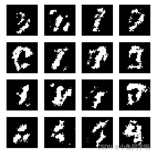
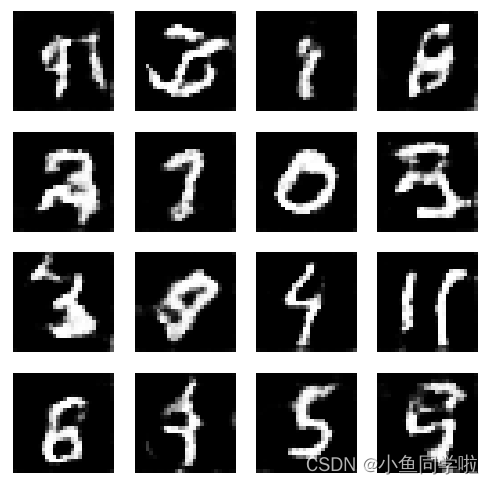
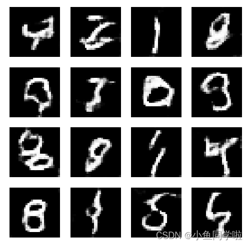
                   epoch=0                                    epoch=5                                   epoch=10

        可以看到虽然只训练了10轮但是效果比原始GAN模型好很多，基本可以肉眼看出具体的数字了。

导入的库：

import torch
import torch.nn as nn
import torch.nn.functional as F
import torch.optim as optim
import numpy as np
import matplotlib.pyplot as plt
import torchvision
from torchvision import transforms
from torch.utils.data import DataLoader

数据准备（这里我们用的是手写数据集MNIST）：

# 数据准备
transform = transforms.Compose([
    transforms.ToTensor(),
    transforms.Normalize(0.5, 0.5)
])
train_ds = torchvision.datasets.MNIST('data', train=True, transform=transform, download=True)
train_dl = DataLoader(train_ds, batch_size=4, shuffle=True)

定义生成器（Generator）：

# 生成器的初始化部分
# PS：1.输出层要用Tanh激活函数  2.使用batchnorm，解决初始化差的问题，帮助梯度传播到每一层，防止生成器包所有的样本都收敛到同一个点
class Generator(nn.Module):
    def __init__(self):
        super(Generator, self).__init__()
        self.linear1 = nn.Linear(100, 256 * 7 * 7)
        self.bn1 = nn.BatchNorm1d(256 * 7 * 7)
        # 这里是反卷积，stride=2即让图像放大2倍,padding=2即往里缩小两格。
        self.decon1 = nn.ConvTranspose2d(in_channels=256, out_channels=128,
                                         kernel_size=(3, 3),
                                         stride=1,
                                         padding=1)  # (128, 7, 7)
        self.bn2 = nn.BatchNorm2d(128)
        self.decon2 = nn.ConvTranspose2d(128, 64,
                                         kernel_size=(4, 4),
                                         stride=2,
                                         padding=1)  # (64, 14, 14)
        self.bn3 = nn.BatchNorm2d(64)
        self.decon3 = nn.ConvTranspose2d(64, 1,
                                         kernel_size=(4, 4),
                                         stride=2,
                                         padding=1)  # (1, 28, 28)

    def forward(self, x):
        x = F.relu(self.linear1(x))
        x = self.bn1(x)
        x = x.view(-1, 256, 7, 7)
        x = F.relu(self.decon1(x))
        x = self.bn2(x)
        x = F.relu(self.decon2(x))
        x = self.bn3(x)
        x = torch.tanh(self.decon3(x))
        return x

定义判别器（Discriminator）：

# 判别器的初始化部分
# PS：1.输入层不能用BN  2.用LeakyReLU激活函数  3.为了防止判别器过强而一边倒，用dropout降低其学习效果
class Discriminator(nn.Module):
    def __init__(self):
        super(Discriminator, self).__init__()
        self.conv1 = nn.Conv2d(in_channels=1, out_channels=64, kernel_size=3, stride=2)
        self.conv2 = nn.Conv2d(in_channels=64, out_channels=128, kernel_size=3, stride=2)
        self.bn = nn.BatchNorm2d(128)
        self.fc = nn.Linear(128 * 6 * 6, 1)

    def forward(self, x):
        x = F.dropout2d(F.leaky_relu_(self.conv1(x)))  # nn.LeakyReLU() 更适合作为模型的一部分使用，因为它会返回一个新的张量，而不会修改原始数据
        x = F.dropout2d(F.leaky_relu_(self.conv2(x)))
        x = self.bn(x)
        x = x.view(-1, 128 * 6 * 6)
        x = self.fc(x)
        return x

初始化模型，定义优化器，损失函数：

# 初始化模型，定义优化器，损失函数
device = 'cuda' if torch.cuda.is_available() else 'cpu'
gen = Generator().to(device)
dis = Discriminator().to(device)
g_optim = optim.Adam(gen.parameters(), lr=1e-4)
d_optim = optim.Adam(dis.parameters(), lr=1e-5)  # PS：将判别器的学习率设置小一点可以减小其学习速度，防止一边倒
loss_fun = torch.nn.MSELoss()

定义绘图函数：

# 定义绘图函数
test_input = torch.randn(16, 100, device=device)


def gen_img_plot(model, test_input):
    prediction = np.squeeze(model(test_input).detach().cpu().numpy())
    plt.figure(figsize=(4, 4))
    for i in range(16):
        plt.subplot(4, 4, i + 1)
        plt.imshow((prediction[i] + 1) / 2, cmap="gray")
        plt.axis("off")
    plt.show()

训练GAN：

# 训练GAN
G_loss = []
D_loss = []
for epoch in range(20):
    g_epoch_loss = 0
    d_epoch_loss = 0
    count = len(train_dl)
    for step, (img, _) in enumerate(train_dl):
        img = img.to(device)
        size = img.size(0)
        random_noise = torch.randn(size, 100, device=device)
        # 优化判别器
        d_optim.zero_grad()
        # 优化真实图片
        real_output = dis(img)
        real_loss = loss_fun(real_output, torch.ones_like(real_output, device=device))
        real_loss.backward()
        # 优化生成图片
        gen_img = gen(random_noise)
        fake_output = dis(gen_img.detach())
        fake_loss = loss_fun(fake_output, torch.zeros_like(fake_output, device=device))
        fake_loss.backward()

        d_loss = real_loss + fake_loss
        d_optim.step()

        # 优化生成器
        g_optim.zero_grad()
        fake_output = dis(gen_img)
        g_loss = loss_fun(fake_output, torch.ones_like(fake_output, device=device))
        g_loss.backward()
        g_optim.step()

        with torch.no_grad():
            d_epoch_loss += d_loss.item()
            g_epoch_loss += g_loss.item()

    with torch.no_grad():
        d_epoch_loss /= count
        g_epoch_loss /= count
        D_loss.append(d_epoch_loss)
        G_loss.append(g_epoch_loss)
        print("Epoch:", epoch)
        gen_img_plot(gen, test_input)

plt.plot(D_loss, label="D_loss")
plt.plot(G_loss, label="G_loss")
plt.legend()
plt.show()

完整代码：

# 训练GAN
G_loss = []
D_loss = []
for epoch in range(20):
    g_epoch_loss = 0
    d_epoch_loss = 0
    count = len(train_dl)
    for step, (img, _) in enumerate(train_dl):
        img = img.to(device)
        size = img.size(0)
        random_noise = torch.randn(size, 100, device=device)
        # 优化判别器
        d_optim.zero_grad()
        # 优化真实图片
        real_output = dis(img)
        real_loss = loss_fun(real_output, torch.ones_like(real_output, device=device))
        real_loss.backward()
        # 优化生成图片
        gen_img = gen(random_noise)
        fake_output = dis(gen_img.detach())
        fake_loss = loss_fun(fake_output, torch.zeros_like(fake_output, device=device))
        fake_loss.backward()

        d_loss = real_loss + fake_loss
        d_optim.step()

        # 优化生成器
        g_optim.zero_grad()
        fake_output = dis(gen_img)
        g_loss = loss_fun(fake_output, torch.ones_like(fake_output, device=device))
        g_loss.backward()
        g_optim.step()

        with torch.no_grad():
            d_epoch_loss += d_loss.item()
            g_epoch_loss += g_loss.item()

    with torch.no_grad():
        d_epoch_loss /= count
        g_epoch_loss /= count
        D_loss.append(d_epoch_loss)
        G_loss.append(g_epoch_loss)
        print("Epoch:", epoch)
        gen_img_plot(gen, test_input)

plt.plot(D_loss, label="D_loss")
plt.plot(G_loss, label="G_loss")
plt.legend()
plt.show()