


CGAN理论讲解:
论文地址:https://arxiv.org/pdf/1411.1784.pdf
说CGAN之前,先让我们聊一聊原始GAN的缺点,毕竟CGAN就是为了解决原始GAN的问题而出现的。原始GAN生成的图像是随机的,不可预测的,无法控制网络输出特定的图片,生成目标不准确,可控性不强。针对原始GAN不能生成具有特定属性的图片的问题,Mehdi Mirza等人提出了今天我们所要讲的CGAN(conditional gan),其核心在于将属性信息y融入生成器和判别器中,属性y可以是任何标签信息,例如图像的类别、人脸图像的面部表情等。
CGAN将 无监督学习 转为 有监督学习,使得网络可以更好的在我们掌控下进行学习。
CGAN损失计算公式:
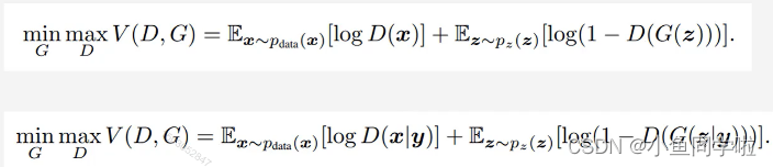
从公式看,CGAN相当于在原始GAN的基础上对生成器部分和判别器部分都加了一个条件y(关于原始GAN的公式可以参见:【对抗网络】Gan的基本公式详解-CSDN博客)
CGAN整体架构:
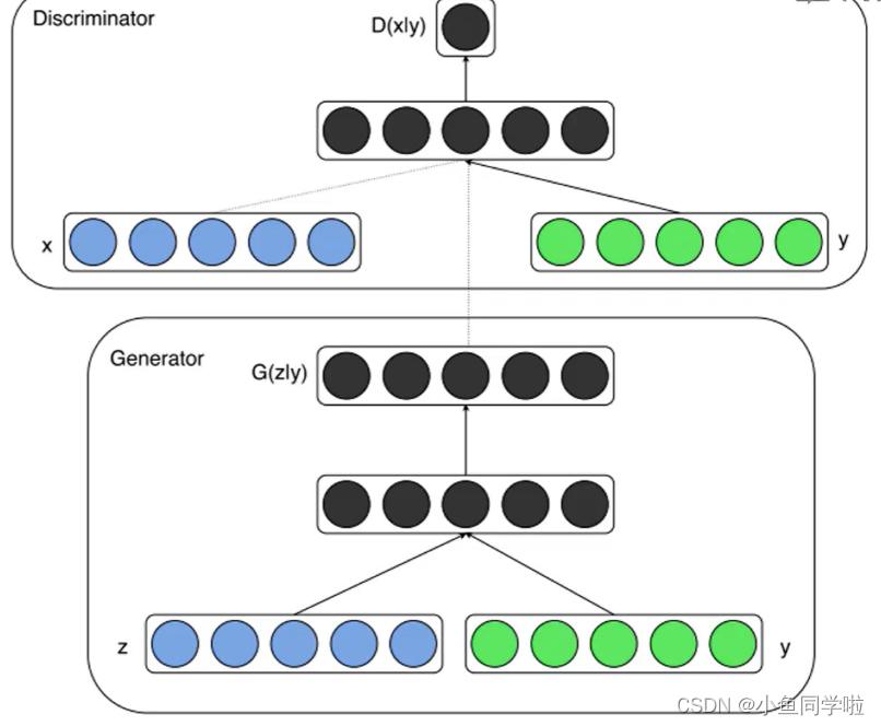
CGAN的中心思想是希望可以控制GAN生成的图片,而不是单纯的随机生成图片。具体来说,Conditinal GAN 在生成器和判别器的输入中增加了额外的信息条件(如上图的绿色信息条件y),生成器生成的图片只有足够真实且与条件相符,才能够通过判别器。
运行结果:
我们指定生成的数字:[ [5, 2, 2, 5], [ 9, 5, 6, 8], [5, 8, 4, 3], [7, 4, 8, 7] ]
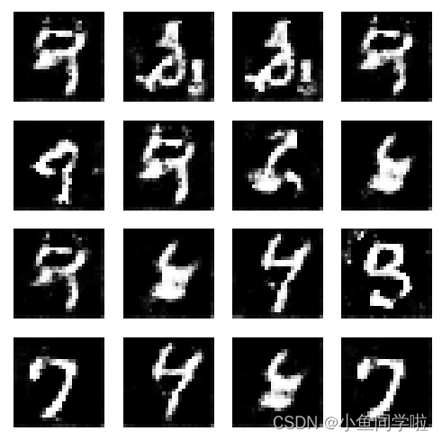
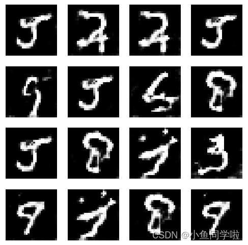
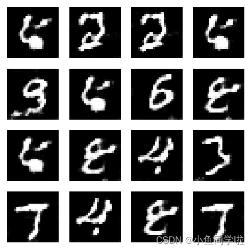
epoch=0 epoch=5 epoch=10
导入的库:
import torch
import torch.nn as nn
import torch.nn.functional as F
from torch.utils import data
import torchvision
from torchvision import transforms

import numpy as np
import matplotlib.pyplot as plt

transform = transforms.Compose([
    transforms.ToTensor(),
    transforms.Normalize(0.5, 0.5)
])
数据准备(这里要用独热编码将标签转换成张量形式):
# 独热编码,将标签转变成张量形式
def one_hot(x, class_count=10):
    return torch.eye(class_count)[x, :]


dataset = torchvision.datasets.MNIST(
    'data', train=True,
    transform=transform,
    target_transform=one_hot)  # target_transform 是一个在数据加载过程中用于对目标(标签)进行预处理的参数

dataloader = data.DataLoader(dataset, batch_size=4, shuffle=True)
生成器的初始化部分:
# 生成器的初始化部分
# PS:1.输出层要用Tanh激活函数  2.使用batchnorm,解决初始化差的问题,帮助梯度传播到每一层,防止生成器包所有的样本都收敛到同一个点
class Generator(nn.Module):
    def __init__(self):
        super(Generator, self).__init__()
        self.linear1 = nn.Linear(100, 128 * 7 * 7)
        self.bn1 = nn.BatchNorm1d(128 * 7 * 7)
        self.linear2 = nn.Linear(10, 128 * 7 * 7)
        self.bn2 = nn.BatchNorm1d(128 * 7 * 7)
        # 这里是反卷积,stride=2即让图像放大2倍,padding=2即往里缩小两格。
        self.decon1 = nn.ConvTranspose2d(in_channels=256, out_channels=128,
                                         kernel_size=(3, 3),
                                         stride=1,
                                         padding=1)  # (128, 7, 7)
        self.bn3 = nn.BatchNorm2d(128)
        self.decon2 = nn.ConvTranspose2d(128, 64,
                                         kernel_size=(4, 4),
                                         stride=2,
                                         padding=1)  # (64, 14, 14)
        self.bn4 = nn.BatchNorm2d(64)
        self.decon3 = nn.ConvTranspose2d(64, 1,
                                         kernel_size=(4, 4),
                                         stride=2,
                                         padding=1)  # (1, 28, 28)

    def forward(self, x1, x2):
        x1 = F.relu(self.linear1(x1))
        x1 = self.bn1(x1)
        x1 = x1.view(-1, 128, 7, 7)
        x2 = F.relu(self.linear2(x2))
        x2 = self.bn2(x2)
        x2 = x2.view(-1, 128, 7, 7)
        x = torch.cat([x1, x2], dim=1)  # batch, 256, 7, 7  用来将两个通道数(dim=1)进行拼接
        x = F.relu(self.decon1(x))
        x = self.bn3(x)
        x = F.relu(self.decon2(x))
        x = self.bn4(x)
        x = torch.tanh(self.decon3(x))
        return x
判别器的初始化部分:
# 判别器的初始化部分
# PS:1.输入层不能用BN  2.用LeakyReLU激活函数  3.为了防止判别器过强而一边倒,用dropout降低其学习效果
# 输入:1.长度为10的噪声  2.(1, 28, 28)的图片
class Discriminator(nn.Module):
    def __init__(self):
        super(Discriminator, self).__init__()
        self.linear = nn.Linear(10, 1 * 28 * 28)
        self.conv1 = nn.Conv2d(in_channels=2, out_channels=64, kernel_size=3, stride=2)
        self.conv2 = nn.Conv2d(in_channels=64, out_channels=128, kernel_size=3, stride=2)
        self.bn = nn.BatchNorm2d(128)
        self.fc = nn.Linear(128 * 6 * 6, 1)

    def forward(self, x1, x2):
        x1 = F.leaky_relu_(self.linear(x1))
        x1 = x1.view(-1, 1, 28, 28)
        x = torch.cat([x1, x2], dim=1)  # shape:batch,2 ,28,28
        x = F.dropout2d(F.leaky_relu_(self.conv1(x)))  # nn.LeakyReLU() 更适合作为模型的一部分使用,因为它会返回一个新的张量,而不会修改原始数据
        x = F.dropout2d(F.leaky_relu_(self.conv2(x)))
        x = self.bn(x)
        x = x.view(-1, 128 * 6 * 6)
        x = torch.sigmoid(self.fc(x))
        return x
初始化模型,定义优化器,损失函数:
# 初始化模型,定义优化器,损失函数
device = 'cuda' if torch.cuda.is_available() else 'cpu'
gen = Generator().to(device)
dis = Discriminator().to(device)
g_optim = torch.optim.Adam(gen.parameters(), lr=0.0001)
d_optim = torch.optim.Adam(dis.parameters(), lr=0.0001)  # PS:将判别器的学习率设置小一点可以减小其学习速度,防止一边倒
loss_fun = torch.nn.BCELoss()
定义绘图函数:
# 定义绘图函数

def gen_img_plot(model, label_input, noise_input):
    prediction = np.squeeze(model(noise_input, label_input).cpu().numpy())
    plt.figure(figsize=(4, 4))
    for i in range(prediction.shape[0]):
        plt.subplot(4, 4, i + 1)
        plt.imshow((prediction[i] + 1) / 2, cmap="gray")
        plt.axis("off")
    plt.show()


noise_seed = torch.randn(16, 100, device=device)
label_seed = torch.randint(0, 10, size=(16,))
label_seed_onehot = one_hot(label_seed).to(device)
print(label_seed)
训练GAN:
# 训练GAN
G_loss = []
D_loss = []
for epoch in range(20):
    g_epoch_loss = 0
    d_epoch_loss = 0
    count = len(dataloader)
    for step, (img, label) in enumerate(dataloader):
        img = img.to(device)
        label = label.to(device)
        size = img.shape[0]
        random_seed = torch.randn(size, 100, device=device)
        # 优化判别器
        d_optim.zero_grad()
        # 优化真实图片
        real_output = dis(label, img)
        real_loss = loss_fun(real_output, torch.ones_like(real_output, device=device))
        real_loss.backward()
        # 优化生成图片
        # print("Label shape:", label.shape)
        # print("Random seed shape:", random_seed.shape)

        gen_img = gen(random_seed, label)
        fake_output = dis(label, gen_img.detach())
        fake_loss = loss_fun(fake_output, torch.zeros_like(fake_output, device=device))
        fake_loss.backward()

        d_loss = real_loss + fake_loss
        d_optim.step()

        # 优化生成器
        g_optim.zero_grad()
        fake_output = dis(label, gen_img)
        g_loss = loss_fun(fake_output, torch.ones_like(fake_output, device=device))
        g_loss.backward()
        g_optim.step()

        with torch.no_grad():
            d_epoch_loss += d_loss.item()
            g_epoch_loss += g_loss.item()

    with torch.no_grad():
        d_epoch_loss /= count
        g_epoch_loss /= count
        D_loss.append(d_epoch_loss)
        G_loss.append(g_epoch_loss)
        print("Epoch:", epoch)
        print(label_seed)
        gen_img_plot(gen, label_seed_onehot, noise_seed)

plt.plot(D_loss, label="D_loss")
plt.plot(G_loss, label="G_loss")
plt.legend()
plt.show()
完整代码:
import torch
import torch.nn as nn
import torch.nn.functional as F
from torch.utils import data
import torchvision
from torchvision import transforms

import numpy as np
import matplotlib.pyplot as plt

transform = transforms.Compose([
    transforms.ToTensor(),
    transforms.Normalize(0.5, 0.5)
])


# 独热编码,将标签转变成张量形式
def one_hot(x, class_count=10):
    return torch.eye(class_count)[x, :]


dataset = torchvision.datasets.MNIST(
    'data', train=True,
    transform=transform,
    target_transform=one_hot)  # target_transform 是一个在数据加载过程中用于对目标(标签)进行预处理的参数

dataloader = data.DataLoader(dataset, batch_size=4, shuffle=True)


# 生成器的初始化部分
# PS:1.输出层要用Tanh激活函数  2.使用batchnorm,解决初始化差的问题,帮助梯度传播到每一层,防止生成器包所有的样本都收敛到同一个点
class Generator(nn.Module):
    def __init__(self):
        super(Generator, self).__init__()
        self.linear1 = nn.Linear(100, 128 * 7 * 7)
        self.bn1 = nn.BatchNorm1d(128 * 7 * 7)
        self.linear2 = nn.Linear(10, 128 * 7 * 7)
        self.bn2 = nn.BatchNorm1d(128 * 7 * 7)
        # 这里是反卷积,stride=2即让图像放大2倍,padding=2即往里缩小两格。
        self.decon1 = nn.ConvTranspose2d(in_channels=256, out_channels=128,
                                         kernel_size=(3, 3),
                                         stride=1,
                                         padding=1)  # (128, 7, 7)
        self.bn3 = nn.BatchNorm2d(128)
        self.decon2 = nn.ConvTranspose2d(128, 64,
                                         kernel_size=(4, 4),
                                         stride=2,
                                         padding=1)  # (64, 14, 14)
        self.bn4 = nn.BatchNorm2d(64)
        self.decon3 = nn.ConvTranspose2d(64, 1,
                                         kernel_size=(4, 4),
                                         stride=2,
                                         padding=1)  # (1, 28, 28)

    def forward(self, x1, x2):
        x1 = F.relu(self.linear1(x1))
        x1 = self.bn1(x1)
        x1 = x1.view(-1, 128, 7, 7)
        x2 = F.relu(self.linear2(x2))
        x2 = self.bn2(x2)
        x2 = x2.view(-1, 128, 7, 7)
        x = torch.cat([x1, x2], dim=1)  # batch, 256, 7, 7  用来将两个通道数(dim=1)进行拼接
        x = F.relu(self.decon1(x))
        x = self.bn3(x)
        x = F.relu(self.decon2(x))
        x = self.bn4(x)
        x = torch.tanh(self.decon3(x))
        return x


# 判别器的初始化部分
# PS:1.输入层不能用BN  2.用LeakyReLU激活函数  3.为了防止判别器过强而一边倒,用dropout降低其学习效果
# 输入:1.长度为10的噪声  2.(1, 28, 28)的图片
class Discriminator(nn.Module):
    def __init__(self):
        super(Discriminator, self).__init__()
        self.linear = nn.Linear(10, 1 * 28 * 28)
        self.conv1 = nn.Conv2d(in_channels=2, out_channels=64, kernel_size=3, stride=2)
        self.conv2 = nn.Conv2d(in_channels=64, out_channels=128, kernel_size=3, stride=2)
        self.bn = nn.BatchNorm2d(128)
        self.fc = nn.Linear(128 * 6 * 6, 1)

    def forward(self, x1, x2):
        x1 = F.leaky_relu_(self.linear(x1))
        x1 = x1.view(-1, 1, 28, 28)
        x = torch.cat([x1, x2], dim=1)  # shape:batch,2 ,28,28
        x = F.dropout2d(F.leaky_relu_(self.conv1(x)))  # nn.LeakyReLU() 更适合作为模型的一部分使用,因为它会返回一个新的张量,而不会修改原始数据
        x = F.dropout2d(F.leaky_relu_(self.conv2(x)))
        x = self.bn(x)
        x = x.view(-1, 128 * 6 * 6)
        x = torch.sigmoid(self.fc(x))
        return x


# 初始化模型,定义优化器,损失函数
device = 'cuda' if torch.cuda.is_available() else 'cpu'
gen = Generator().to(device)
dis = Discriminator().to(device)
g_optim = torch.optim.Adam(gen.parameters(), lr=0.0001)
d_optim = torch.optim.Adam(dis.parameters(), lr=0.0001)  # PS:将判别器的学习率设置小一点可以减小其学习速度,防止一边倒
loss_fun = torch.nn.BCELoss()


# 定义绘图函数

def gen_img_plot(model, label_input, noise_input):
    prediction = np.squeeze(model(noise_input, label_input).cpu().numpy())
    plt.figure(figsize=(4, 4))
    for i in range(prediction.shape[0]):
        plt.subplot(4, 4, i + 1)
        plt.imshow((prediction[i] + 1) / 2, cmap="gray")
        plt.axis("off")
    plt.show()


noise_seed = torch.randn(16, 100, device=device)
label_seed = torch.randint(0, 10, size=(16,))
label_seed_onehot = one_hot(label_seed).to(device)
print(label_seed)

# 训练GAN
G_loss = []
D_loss = []
for epoch in range(20):
    g_epoch_loss = 0
    d_epoch_loss = 0
    count = len(dataloader)
    for step, (img, label) in enumerate(dataloader):
        img = img.to(device)
        label = label.to(device)
        size = img.shape[0]
        random_seed = torch.randn(size, 100, device=device)
        # 优化判别器
        d_optim.zero_grad()
        # 优化真实图片
        real_output = dis(label, img)
        real_loss = loss_fun(real_output, torch.ones_like(real_output, device=device))
        real_loss.backward()
        # 优化生成图片
        # print("Label shape:", label.shape)
        # print("Random seed shape:", random_seed.shape)

        gen_img = gen(random_seed, label)
        fake_output = dis(label, gen_img.detach())
        fake_loss = loss_fun(fake_output, torch.zeros_like(fake_output, device=device))
        fake_loss.backward()

        d_loss = real_loss + fake_loss
        d_optim.step()

        # 优化生成器
        g_optim.zero_grad()
        fake_output = dis(label, gen_img)
        g_loss = loss_fun(fake_output, torch.ones_like(fake_output, device=device))
        g_loss.backward()
        g_optim.step()

        with torch.no_grad():
            d_epoch_loss += d_loss.item()
            g_epoch_loss += g_loss.item()

    with torch.no_grad():
        d_epoch_loss /= count
        g_epoch_loss /= count
        D_loss.append(d_epoch_loss)
        G_loss.append(g_epoch_loss)
        print("Epoch:", epoch)
        print(label_seed)
        gen_img_plot(gen, label_seed_onehot, noise_seed)

plt.plot(D_loss, label="D_loss")
plt.plot(G_loss, label="G_loss")
plt.legend()
plt.show()


 3万+
3万+


 被折叠的 条评论
为什么被折叠?
被折叠的 条评论
为什么被折叠?
 到【灌水乐园】发言


