A Simple Guide to the Versions of the Inception Network

The Inception network was an important milestone in the development of CNN classifiers. Prior to its inception (pun intended), most popular CNNs just stacked convolution layers deeper and deeper, hoping to get better performance.

Designing CNNs in a nutshell. Fun fact, this meme was referenced in the first inception net paper.

The Inception network on the other hand, was complex (heavily engineered). It used a lot of tricks to push performance; both in terms of speed and accuracy. Its constant evolution lead to the creation of several versions of the network. The popular versions are as follows:

• Inception v1.
• Inception v2 and Inception v3.
• Inception v4 and Inception-ResNet.

Each version is an iterative improvement over the previous one. Understanding the upgrades can help us to build custom classifiers that are optimized both in speed and accuracy. Also, depending on your data, a lower version may actually work better.

This blog post aims to elucidate the evolution of the inception network.

Inception v1

This is where it all started. Let us analyze what problem it was purported to solve, and how it solved it. (Paper)

The Premise:

• Salient parts in the image can have extremely large variation in size. For instance, an image with a dog can be either of the following, as shown below. The area occupied by the dog is different in each image.

From left: A dog occupying most of the image, a dog occupying a part of it, and a dog occupying very little space (Images obtained from Unsplash).

• Because of this huge variation in the location of the information, choosing the right kernel size for the convolution operation becomes tough. A larger kernel is preferred for information that is distributed more globally, and a smaller kernel is preferred for information that is distributed more locally.
• Very deep networks are prone to overfitting. It also hard to pass gradient updates through the entire network.
• Naively stacking large convolution operations is computationally expensive.

The Solution:

Why not have filters with multiple sizes operate on the same level? The network essentially would get a bit “wider” rather than “deeper”. The authors designed the inception module to reflect the same.

The below image is the “naive” inception module. It performs convolution on an input, with 3 different sizes of filters (1x1, 3x3, 5x5). Additionally, max pooling is also performed. The outputs are concatenated and sent to the next inception module.

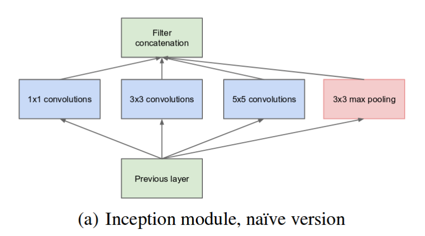
The naive inception module. (Source: Inception v1)

As stated before, deep neural networks are computationally expensive. To make it cheaper, the authors limit the number of input channels by adding an extra 1x1 convolution before the 3x3 and 5x5 convolutions. Though adding an extra operation may seem counterintuitive, 1x1 convolutions are far more cheaper than 5x5 convolutions, and the reduced number of input channels also help. Do note that however, the 1x1 convolution is introduced after the max pooling layer, rather than before.

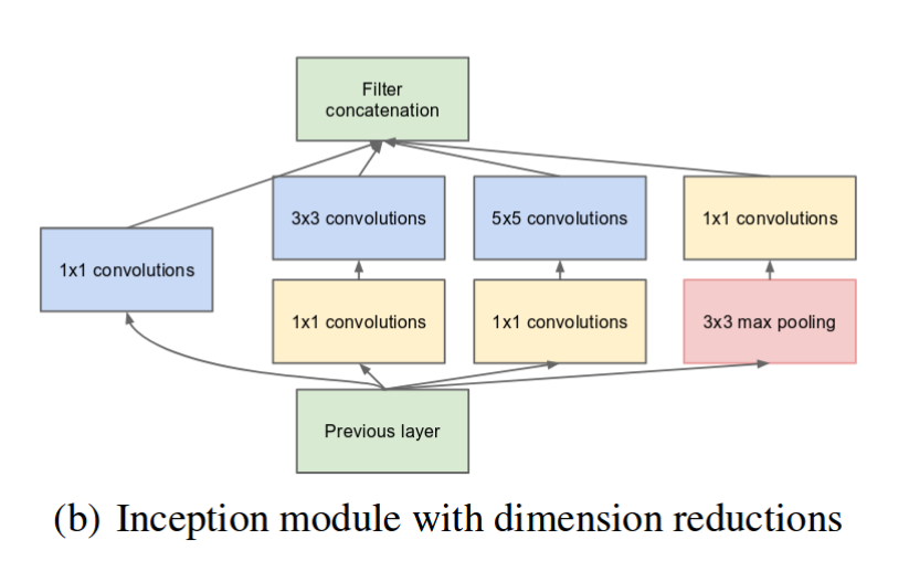
Inception module with dimension reduction. (Source: Inception v1)

Using the dimension reduced inception module, a neural network architecture was built. This was popularly known as GoogLeNet (Inception v1). The architecture is shown below:

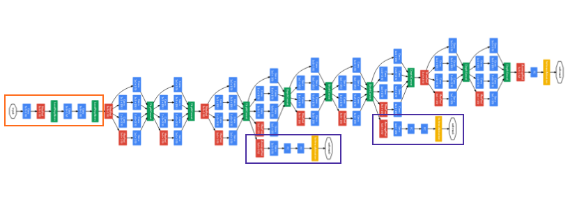
GoogLeNet. The orange box is the stem, which has some preliminary convolutions. The purple boxes are auxiliary classifiers. The wide parts are the inception modules. (Source: Inception v1)

GoogLeNet has 9 such inception modules stacked linearly. It is 22 layers deep (27, including the pooling layers). It uses global average pooling at the end of the last inception module.

Needless to say, it is a pretty deep classifier. As with any very deep network, it is subject to the vanishing gradient problem.

To prevent the middle part of the network from “dying out”, the authors introduced two auxiliary classifiers (The purple boxes in the image). They essentially applied softmax to the outputs of two of the inception modules, and computed an auxiliary loss over the same labels. The total loss functionis a weighted sum of the auxiliary loss and the real loss. Weight value used in the paper was 0.3 for each auxiliary loss.

# The total loss used by the inception net during training.
total_loss = real_loss + 0.3 * aux_loss_1 + 0.3 * aux_loss_2

Needless to say, auxiliary loss is purely used for training purposes, and is ignored during inference.

Inception v2

Inception v2 and Inception v3 were presented in the same paper. The authors proposed a number of upgrades which increased the accuracy and reduced the computational complexity. Inception v2 explores the following:

The Premise:

• Reduce representational bottleneck. The intuition was that, neural networks perform better when convolutions didn’t alter the dimensions of the input drastically. Reducing the dimensions too much may cause loss of information, known as a “representational bottleneck”
• Using smart factorization methods, convolutions can be made more efficient in terms of computational complexity.

The Solution:

• Factorize 5x5 convolution to two 3x3 convolution operations to improve computational speed. Although this may seem counterintuitive, a 5x5 convolution is 2.78 times more expensive than a 3x3 convolution. So stacking two 3x3 convolutions infact leads to a boost in performance. This is illustrated in the below image.

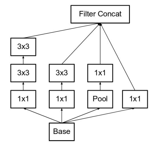
The left-most 5x5 convolution of the old inception module, is now represented as two 3x3 convolutions. (Source: Incpetion v2)

• Moreover, they factorize convolutions of filter size nxn to a combinationof 1xn and nx1 convolutions. For example, a 3x3 convolution is equivalent to first performing a 1x3 convolution, and then performing a 3x1 convolution on its output. They found this method to be 33% more cheaper than the single 3x3 convolution. This is illustrated in the below image.

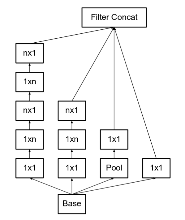
Here, put n=3 to obtain the equivalent of the previous image. The left-most 5x5 convolution can be represented as two 3x3 convolutions, which inturn are represented as 1x3 and 3x1 in series. (Source: Incpetion v2)

• The filter banks in the module were expanded (made wider instead of deeper) to remove the representational bottleneck. If the module was made deeper instead, there would be excessive reduction in dimensions, and hence loss of information. This is illustrated in the below image.

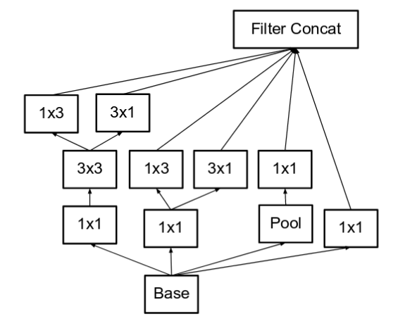
Making the inception module wider. This type is equivalent to the module shown above. (Source: Incpetion v2)

• The above three principles were used to build three different types of inception modules (Let’s call them modules A,B and C in the order they were introduced. These names are introduced for clarity, and not the official names). The architecture is as follows:

Here, “figure 5” is module A, “figure 6” is module B and “figure 7” is module C. (Source: Incpetion v2)

Inception v3

The Premise

• The authors noted that the auxiliary classifiers didn’t contribute much until near the end of the training process, when accuracies were nearing saturation. They argued that they function as regularizes, especially if they have BatchNorm or Dropout operations.
• Possibilities to improve on the Inception v2 without drastically changing the modules were to be investigated.

The Solution

• Inception Net v3 incorporated all of the above upgrades stated for Inception v2, and in addition used the following:

1. RMSProp Optimizer.
2. Factorized 7x7 convolutions.
3. BatchNorm in the Auxillary Classifiers.
4. Label Smoothing (A type of regularizing component added to the loss formula that prevents the network from becoming too confident about a class. Prevents over fitting).

Inception v4

Inception v4 and Inception-ResNet were introduced in the same paper. For clarity, let us discuss them in separate sections.

The Premise

• Make the modules more uniform. The authors also noticed that some of the modules were more complicated than necessary. This can enable us to boost performance by adding more of these uniform modules.

The Solution

• The “stem” of Inception v4 was modified. The stem here, refers to the initial set of operations performed before introducing the Inception blocks.

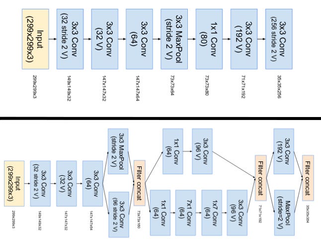
The top image is the stem of Inception-ResNet v1. The bottom image is the stem of Inception v4 and Inception-ResNet v2. (Source: Inception v4)

• They had three main inception modules, named A,B and C (Unlike Inception v2, these modules are infact named A,B and C). They look very similar to their Inception v2 (or v3) counterparts.

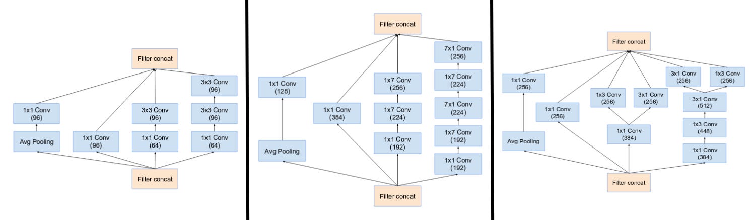
(From left) Inception modules A,B,C used in Inception v4. Note how similar they are to the Inception v2 (or v3) modules. (Source: Inception v4)

• Inception v4 introduced specialized “Reduction Blocks” which are used to change the width and height of the grid. The earlier versions didn’t explicitly have reduction blocks, but the functionality was implemented.

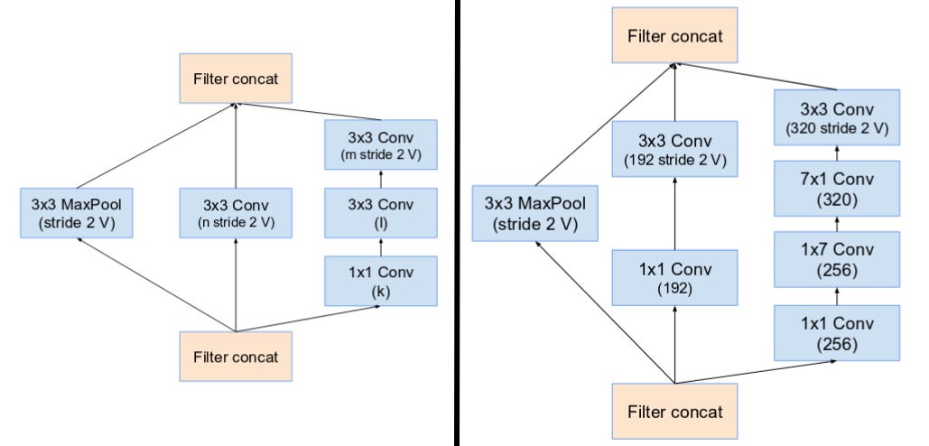
(From Left) Reduction Block A (35x35 to 17x17 size reduction) and Reduction Block B (17x17 to 8x8 size reduction). Refer to the paper for the exact hyper-parameter setting (V,l,k). (Source: Inception v4)

Inception-ResNet v1 and v2

Inspired by the performance of the ResNet, a hybrid inception module was proposed. There are two sub-versions of Inception ResNet, namely v1 and v2. Before we checkout the salient features, let us look at the minor differences between these two sub-versions.

• Inception-ResNet v1 has a computational cost that is similar to that of Inception v3.
• Inception-ResNet v2 has a computational cost that is similar to that of Inception v4.
• They have different stems, as illustrated in the Inception v4 section.
• Both sub-versions have the same structure for the modules A, B, C and the reduction blocks. Only difference is the hyper-parameter settings. In this section, we’ll only focus on the structure. Refer to the paper for the exact hyper-parameter settings (The images are of Inception-Resnet v1).

The Premise

• Introduce residual connections that add the output of the convolution operation of the inception module, to the input.

The Solution

• For residual addition to work, the input and output after convolution must have the same dimensions. Hence, we use 1x1 convolutions after the original convolutions, to match the depth sizes (Depth is increased after convolution).

(From left) Inception modules A,B,C in an Inception ResNet. Note how the pooling layer was replaced by the residual connection, and also the additional 1x1 convolution before addition. (Source: Inception v4)

• The pooling operation inside the main inception modules were replaced in favor of the residual connections. However, you can still find those operations in the reduction blocks. Reduction block A is same as that of Inception v4.

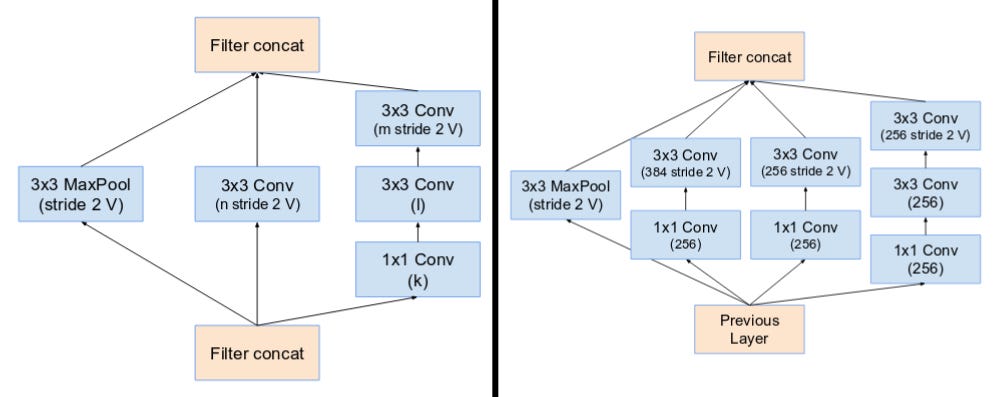
(From Left) Reduction Block A (35x35 to 17x17 size reduction) and Reduction Block B (17x17 to 8x8 size reduction). Refer to the paper for the exact hyper-parameter setting (V,l,k). (Source: Inception v4)

• Networks with residual units deeper in the architecture caused the network to “die” if the number of filters exceeded 1000. Hence, to increase stability, the authors scaled the residual activations by a value around 0.1 to 0.3.

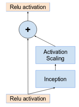
Activations are scaled by a constant to prevent the network from dying. (Source: Inception v4)

• The original paper didn’t use BatchNorm after summation to train the model on a single GPU (To fit the entire model on a single GPU).
• It was found that Inception-ResNet models were able to achieve higher accuracies at a lower epoch.
• The final network layout for both Inception v4 and Inception-ResNet are as follows:

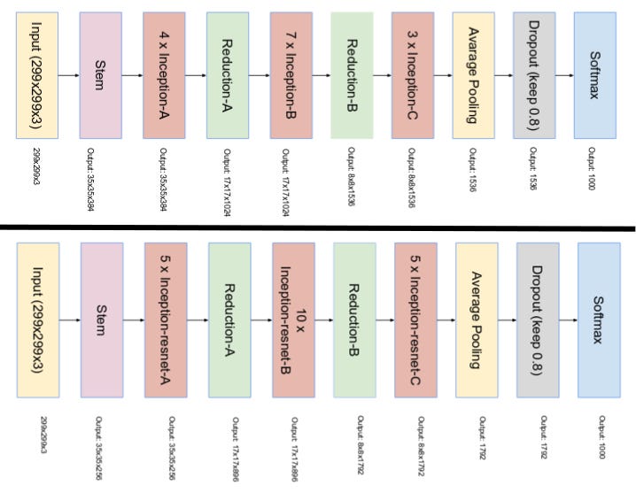
The top image is the layout of Inception v4. The bottom image is the layout of Inception-ResNet. (Source: Inception v4)

---

Thank you for reading this article! Hope it gave you some clarity about the the Inception Net. Hit the clap button if it did! If you have any questions, you could hit me up on  social media or send me an email (bharathrajn98@gmail.com).