深入解析强化学习中的 Generalized Advantage Estimation (GAE)

中文版

深入解析强化学习中的 Generalized Advantage Estimation (GAE)

---

1. 什么是 Generalized Advantage Estimation (GAE)?

在强化学习中，计算策略梯度的关键在于 优势函数（Advantage Function） 的设计。优势函数 ( $A(s,a)$ ) 衡量了执行某动作 ( $a$ ) 比其他动作的相对价值。然而，优势函数的估计往往面临以下两大问题：

1. 高方差问题：由于强化学习中的样本通常有限，直接使用单步回报或 Monte Carlo 方法计算优势值会导致高方差。
2. 偏差问题：使用引入近似函数（如值函数 ( $V(s)$ )）会降低方差，但可能引入偏差。

为了平衡 偏差和方差，Schulman 等人在 2016 年提出了 Generalized Advantage Estimation (GAE) 方法，它是一种在偏差和方差之间权衡的优势函数估计方法，被广泛应用于强化学习中的近端策略优化（PPO）等算法。

---

2. GAE 的数学原理

GAE 的核心思想是通过时间差分（Temporal Difference, TD）误差的加权和，估计优势函数：

TD 残差（Temporal Difference Residuals）：
$${\delta }_t=r_t+\gamma V(s_{t+1})-V(s_t)$$

GAE 的递归定义：
$$A_t^{\text{GAE}}=\sum _{l=0}^{\infty }(\gamma \lambda {)}^l{\delta }_{t+l}$$

其中：

• ( $\gamma$ ) 是折扣因子，用于控制未来回报的权重。
• ( $\lambda$ ) 是 GAE 的衰减系数，控制长期和短期偏差的平衡。
• ( ${\delta }_t$ ) 是每一步的 TD 残差，反映即时回报和值函数的差异。

GAE 的公式可以通过递归形式表示为：
$$A_t^{\text{GAE}}={\delta }_t+(\gamma \lambda )\cdot A_{t+1}^{\text{GAE}}$$

通过 ( $\lambda$ ) 的调节，GAE 可以在单步 TD 估计（低方差高偏差）和 Monte Carlo 估计（高方差低偏差）之间找到一个平衡点。

---

3. GAE 在 PPO 中的应用

PPO paper：https://arxiv.org/pdf/1707.06347

在近端策略优化（PPO）算法中，策略梯度的更新依赖于优势函数 ( $A_t$ ) 的估计，而 GAE 为优势函数的估计提供了一个高效的工具。

PPO 的 损失函数 包括两部分：

1. 策略更新（Actor Loss）：
   $$L^{\text{actor}}={\mathbb{E}}_t\left[\min (r_t(\theta )\cdot A_t^{\text{GAE}},\text{clip}(r_t(\theta ),1-ϵ,1+ϵ)\cdot A_t^{\text{GAE}})\right]$$
   其中 ( $r_t(\theta )$ ) 是当前策略与旧策略的概率比。

2. 值函数更新（Critic Loss）：
   $$L^{\text{critic}}={\mathbb{E}}_t\left[(R_t-V(s_t){)}^2\right]$$

PPO 使用 GAE 来高效估计 ( $A_t$ )，从而使得梯度更新既稳定又高效。

---

4. GAE 的代码实现

以下是 GAE 的核心代码实现：

import numpy as np

def compute_gae(rewards, values, gamma=0.99, lam=0.95):
    """
    使用 GAE 计算优势函数
    Args:
        rewards: 每一步的即时奖励 (list or array)
        values: 每一步的状态值函数估计 (list or array)
        gamma: 折扣因子
        lam: GAE 的衰减系数
    Returns:
        advantages: 每一步的优势函数估计
    """
    advantages = np.zeros_like(rewards)
    gae = 0  # 初始化 GAE
    for t in reversed(range(len(rewards))):
        delta = rewards[t] + gamma * (values[t + 1] if t < len(rewards) - 1 else 0) - values[t]
        gae = delta + gamma * lam * gae
        advantages[t] = gae
    return advantages

# 示例数据
rewards = [1, 1, 1, 1, 1]  # 即时奖励
values = [0.5, 0.6, 0.7, 0.8, 0.9]  # 状态值函数估计
advantages = compute_gae(rewards, values)
print("GAE 计算结果:", advantages)

---

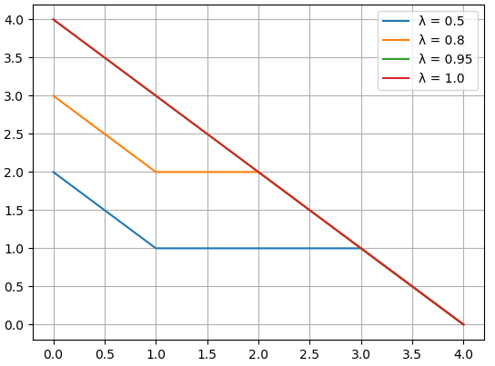
5. 数值模拟

假设我们有以下场景：

• 即时奖励：玩家在每一步获得固定奖励 ( $r_t=1$ )。
• 状态值估计：模型估计的值函数逐步递增。

我们将模拟不同 ( $\lambda$ ) 值对优势函数估计的影响。

import matplotlib.pyplot as plt

# 参数设置
gamma = 0.99
rewards = [1, 1, 1, 1, 1]
values = [0.5, 0.6, 0.7, 0.8, 0.9]

# 不同 lambda 值的 GAE
lambda_values = [0.5, 0.8, 0.95, 1.0]
results = {}

for lam in lambda_values:
    advantages = compute_gae(rewards, values, gamma, lam)
    results[lam] = advantages

# 绘图
for lam, adv in results.items():
    plt.plot(adv, label=f"λ = {lam}")

plt.xlabel("时间步 (t)")
plt.ylabel("优势函数 (A_t)")
plt.title("不同 λ 对 GAE 的影响")
plt.legend()
plt.grid()
plt.show()

绘图结果

---

6. 总结

1. GAE 的优势：

   • 低方差：通过 ( $\lambda$ ) 控制，引入更多的短期回报，减少方差。
   • 高效率：兼顾短期 TD 和长期 Monte Carlo 的优点。
   • 灵活性：可以根据任务需求调整偏差和方差的权衡。

2. PPO 中的应用：
   GAE 是 PPO 算法中计算优势函数的重要工具，其估计结果直接影响策略梯度和价值函数的更新效率。

通过本文的介绍，我们可以更深入地理解 GAE 的数学原理、代码实现以及其在实际场景中的应用，希望对强化学习爱好者有所帮助！

英文版

Deep Dive into Generalized Advantage Estimation (GAE) in Reinforcement Learning

---

1. What is Generalized Advantage Estimation (GAE)?

In reinforcement learning, estimating the advantage function ( $A(s,a)$ ) is a crucial step in computing the policy gradient. The advantage function measures how much better a specific action ( a ) is compared to others in a given state ( $s$ ). However, estimating this function poses two main challenges:

1. High variance: Direct computation using one-step rewards or Monte Carlo rollouts often results in high variance, which makes optimization unstable.
2. Bias: Introducing approximations (e.g., using value functions ( $V(s)$ )) reduces variance but introduces bias.

To balance bias and variance, Schulman et al. introduced Generalized Advantage Estimation (GAE) in 2016. GAE is an efficient method that adjusts the advantage function estimate using a weighted sum of temporal difference (TD) residuals.

---

2. Mathematical Foundation of GAE

The key idea of GAE is to compute the advantage function using a combination of short-term and long-term rewards, weighted by a decay factor.

Temporal Difference (TD) Residual:
$${\delta }_t=r_t+\gamma V(s_{t+1})-V(s_t)$$

GAE Recursive Formula:
$$A_t^{\text{GAE}}=\sum _{l=0}^{\infty }(\gamma \lambda {)}^l{\delta }_{t+l}$$

Where:

• ( $\gamma$ ) is the discount factor, controlling the weight of future rewards.
• ( $\lambda$ ) is the GAE decay factor, balancing short-term and long-term contributions.
• ( ${\delta }_t$ ) is the TD residual, representing the difference between immediate rewards and value estimates.

Alternatively, GAE can be written recursively:
$$A_t^{\text{GAE}}={\delta }_t+(\gamma \lambda )\cdot A_{t+1}^{\text{GAE}}$$

By adjusting ( $\lambda$ ), GAE can interpolate between:

• Low variance, high bias: ( $\lambda =0$ ) (one-step TD residual).
• High variance, low bias: ( $\lambda =1$ ) (Monte Carlo return).

---

3. Application of GAE in PPO

In Proximal Policy Optimization (PPO), GAE plays a critical role in estimating the advantage function, which is used in both the policy update and value function update.

PPO Loss Function:

1. Actor Loss (Policy Update):
   $$L^{\text{actor}}={\mathbb{E}}_t\left[\min (r_t(\theta )\cdot A_t^{\text{GAE}},\text{clip}(r_t(\theta ),1-ϵ,1+ϵ)\cdot A_t^{\text{GAE}})\right]$$
   Where ( $r_t(\theta )$ ) is the probability ratio between the new and old policies.

2. Critic Loss (Value Function Update):
   $$L^{\text{critic}}={\mathbb{E}}_t\left[(R_t-V(s_t){)}^2\right]$$

PPO relies on GAE to provide a stable and accurate advantage estimate ( $A_t^{\text{GAE}}$ ), ensuring efficient policy gradient updates.

---

4. Code Implementation

Below is a Python implementation of GAE:

import numpy as np

def compute_gae(rewards, values, gamma=0.99, lam=0.95):
    """
    Compute Generalized Advantage Estimation (GAE).
    Args:
        rewards: List of rewards at each timestep.
        values: List of value function estimates at each timestep.
        gamma: Discount factor.
        lam: GAE decay factor.
    Returns:
        advantages: GAE-based advantage estimates.
    """
    advantages = np.zeros_like(rewards)
    gae = 0  # Initialize GAE
    for t in reversed(range(len(rewards))):
        delta = rewards[t] + gamma * (values[t + 1] if t < len(rewards) - 1 else 0) - values[t]
        gae = delta + gamma * lam * gae
        advantages[t] = gae
    return advantages

# Example usage
rewards = [1, 1, 1, 1, 1]  # Reward at each timestep
values = [0.5, 0.6, 0.7, 0.8, 0.9]  # Value function estimates
advantages = compute_gae(rewards, values)
print("GAE Advantages:", advantages)
# GAE 计算结果: [4 3 2 1 0]

---

5. Numerical Simulation

We can simulate how different values of ( $\lambda$ ) impact the GAE estimates using the following script:

import matplotlib.pyplot as plt

# Parameters
gamma = 0.99
rewards = [1, 1, 1, 1, 1]
values = [0.5, 0.6, 0.7, 0.8, 0.9]

# Compute GAE for different lambda values
lambda_values = [0.5, 0.8, 0.95, 1.0]
results = {}

for lam in lambda_values:
    advantages = compute_gae(rewards, values, gamma, lam)
    results[lam] = advantages

# Plot the results
for lam, adv in results.items():
    plt.plot(adv, label=f"λ = {lam}")

plt.xlabel("Time Step (t)")
plt.ylabel("Advantage (A_t)")
plt.title("Impact of λ on GAE")
plt.legend()
plt.grid()
plt.show()

---

6. Summary

1. What GAE Solves:

   • GAE balances the bias-variance trade-off in advantage estimation, making it a key tool in reinforcement learning.

2. GAE in PPO:

   • GAE ensures stable and efficient policy updates by providing accurate advantage estimates for the actor-critic framework.

3. Key Takeaways:

   • ( $\lambda$ ) is a critical hyperparameter in GAE, allowing control over the trade-off between bias and variance.
   • GAE is widely adopted in modern reinforcement learning algorithms, particularly in on-policy methods like PPO.

---

This blog post illustrates the importance of GAE in reinforcement learning, along with its implementation and impact on training stability. By leveraging GAE, algorithms like PPO achieve superior performance in complex environments.

后记

2024年12月12日21点38分于上海，在GPT4o大模型辅助下完成。