Flow-GRPO：将在线强化学习融入Flow Matching模型的创新

Flow-GRPO：将在线强化学习融入Flow Matching模型的创新

近年来，Flow Matching模型因其在图像生成领域的强大性能和理论基础而备受关注。然而，在处理复杂场景（如多物体、属性和关系的组合）以及文本渲染任务时，这些模型仍面临挑战。与此同时，在线强化学习（RL），特别是Group Relative Policy Optimization（GRPO），已在提升大语言模型推理能力方面展现出显著效果。论文《Flow-GRPO: Training Flow Matching Models via Online RL》首次将在线RL（具体为GRPO）与Flow Matching模型结合，提出了Flow-GRPO方法，显著提升了文本到图像（T2I）生成任务的表现。本文将面向熟悉Flow Matching和GRPO的读者，介绍Flow-GRPO的贡献、结合方式、解决的关键问题以及核心数学公式。

Paper: https://arxiv.org/pdf/2505.05470

Flow-GRPO的主要贡献

Flow-GRPO的贡献可以总结为以下三点：

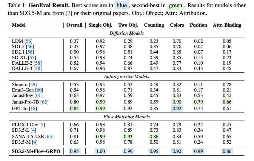
1. 首次将GRPO引入Flow Matching模型：通过将确定性的ODE（常微分方程）采样转换为SDE（随机微分方程）采样，Flow-GRPO克服了Flow Matching模型的确定性限制，使在线RL能够应用于T2I任务。实验表明，Flow-GRPO将Stable Diffusion 3.5 Medium（SD3.5-M）在GenEval基准上的准确率从63%提升至95%，超越了GPT-4o的性能。

2. 去噪步骤减少策略：Flow-GRPO提出了一种Denoising Reduction策略，在训练时减少去噪步骤（从40步降至10步），而在推理时保留完整去噪步骤（40步）。这显著提高了训练效率，同时保持了推理时的图像质量。

3. KL约束防止奖励黑客：通过引入Kullback-Leibler（KL）散度约束，Flow-GRPO有效避免了奖励黑客（reward hacking）现象，即奖励提升但图像质量或多样性下降。实验表明，适当的KL正则化能够在保持任务性能的同时，维护图像质量和生成多样性。

Flow Matching与GRPO的结合方式

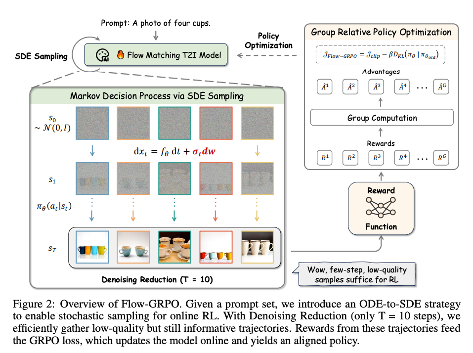
Flow Matching模型通过学习连续时间归一化流的向量场，实现高效的确定性采样。GRPO是一种轻量级在线RL算法，通过组内奖励归一化估计优势（advantage），避免了传统PPO算法中需要额外值函数网络的开销。Flow-GRPO将两者结合，核心思想是将Flow Matching的去噪过程建模为一个马尔可夫决策过程（MDP），并利用GRPO优化生成策略，使其最大化特定任务的奖励（如GenEval的准确率或PickScore的人类偏好分数）。

结合的具体步骤

1. 去噪过程建模为MDP：论文将Flow Matching的去噪过程定义为一个MDP，其中：

   • 状态 ( $s_t=(c,t,x_t)$ )，包括提示词 ( $c$ )、时间步 ( $t$ ) 和当前噪声样本 ( $x_t$ )。
   • 动作 ( $a_t=x_{t-1}$ )，为网络预测的去噪样本。
   • 策略 ( $\pi (a_t|s_t)=p_{\theta }(x_{t-1}|x_t,c)$ )，为条件概率模型。
   • 奖励仅在最后一步非零：( $R(s_t,a_t)=r(x_0,c)$ )（当 ( $t=0$ ) 时），否则为0。

2. GRPO优化：Flow-GRPO基于GRPO框架，优化以下正则化目标：
   $$\underset{\theta }{\max }{\mathbb{E}}_{\left(s_0,a_0,\dots ,s_T,a_T\right)\sim {\pi }_{\theta }}\left[\sum _{t=0}^T\left(R(s_t,a_t)-\beta D_{\mathrm{KL}}\left({\pi }_{\theta }(\cdot |s_t)\Vert {\pi }_{\text{ref}}(\cdot |s_t)\right)\right)\right]$$
   其中，( $\beta$ ) 控制KL散度正则化强度，( ${\pi }_{\text{ref}}$ ) 为参考策略（通常为预训练模型）。GRPO通过组内奖励归一化计算优势：
   A ^ t i = R ( x 0 i , c ) − mean ( { R ( x 0 i , c ) } i = 1 G ) std ( { R ( x 0 i , c ) } i = 1 G ) \hat{A}_t^i = \frac{R(x_0^i, c) - \text{mean}(\{R(x_0^i, c)\}_{i=1}^G)}{\text{std}(\{R(x_0^i, c)\}_{i=1}^G)} A^ti​=std({R(x0i​,c)}i=1G​)R(x0i​,c)−mean({R(x0i​,c)}i=1G​)​
   最终优化目标为：
   F Flow-GRPO ( θ ) = E c ∼ C , { x i } i = 1 G ∼ π θ old ( ⋅ ∣ c ) [ 1 G ∑ i = 1 G 1 T ∑ t = 0 T − 1 ( min ⁡ ( r t i ( θ ) A ^ t i , clip ( r t i ( θ ) , 1 − ε , 1 + ε ) A ^ t i ) − β D K L ( π θ ∥ π ref ) ) ] \mathcal{F}_{\text{Flow-GRPO}}(\theta) = \mathbb{E}_{c \sim \mathcal{C}, \{x^i\}_{i=1}^G \sim \pi_{\theta_{\text{old}}}(\cdot | c)} \left[ \frac{1}{G} \sum_{i=1}^G \frac{1}{T} \sum_{t=0}^{T-1} \left( \min \left( r_t^i(\theta) \hat{A}_t^i, \text{clip}(r_t^i(\theta), 1-\varepsilon, 1+\varepsilon) \hat{A}_t^i \right) - \beta D_{\mathrm{KL}}(\pi_\theta \| \pi_{\text{ref}}) \right) \right] FFlow-GRPO​(θ)=Ec∼C,{xi}i=1G​∼πθold​​(⋅∣c)​[G1​i=1∑G​T1​t=0∑T−1​(min(rti​(θ)A^ti​,clip(rti​(θ),1−ε,1+ε)A^ti​)−βDKL​(πθ​∥πref​))]
   其中，( $r_t^i(\theta )=\frac{p_{\theta }(x_{t-1}^i|x_t^i,c)}{p_{{\theta }_{\text{old}}}(x_{t-1}^i|x_t^i,c)}$ )。

3. 核心策略：

   • ODE-to-SDE转换：为引入随机性以支持RL探索，Flow-GRPO将确定性ODE采样转换为等效的SDE采样，保持边际分布一致。
   • Denoising Reduction：训练时使用较少的去噪步骤（( $T=10$ )），推理时使用完整步骤（( $T=40$ )），加速数据收集。

解决的关键问题

将GRPO应用于Flow Matching模型面临两大挑战：

1. 确定性与随机性的冲突：

   • 问题：Flow Matching依赖确定性ODE采样（公式如下），无法提供RL所需的随机探索和概率计算：
     $$\mathrm{d}{\mathbf{x}}_t={\mathbf{v}}_t\mathrm{d}t$$
     其中，( ${\mathbf{v}}_t$ ) 为通过Flow Matching目标学习的向量场(就是下面的$v$)：
     $$\mathcal{L}(\theta )={\mathbb{E}}_{t,x_0\sim X_0,x_1\sim X_1}\left[{\Vert v-v_{\theta }({\mathbf{x}}_t,t)\Vert }^2\right]$$
     确定性采样（如欧拉法）生成单一轨迹，无法计算 ( $p(x_{t-1}|x_t,c)$ )，也缺乏探索多样性。
   • 解决方案：Flow-GRPO通过ODE-to-SDE转换引入随机性，构造等效SDE：
     $$\mathrm{d}{\mathbf{x}}_t=\left({\mathbf{v}}_t({\mathbf{x}}_t)-\frac{{\sigma }_t^2}{2}\nabla \log p_t({\mathbf{x}}_t)\right)\mathrm{d}t+{\sigma }_t\mathrm{d}\mathbf{w}$$
     其中，($\mathrm{d}\mathbf{w}$ ) 为维纳过程增量，( ${\sigma }_t$ ) 控制随机性。关键在于计算边际分数 ( $\nabla \log p_t({\mathbf{x}}_t)$ )，对于Rectified Flow，论文推导：
     $$\nabla \log p_t(\mathbf{x})=-\frac{\mathbf{x}}{t}-\frac{1-t}{t}{\mathbf{v}}_t(\mathbf{x})$$
     代入后得到最终SDE：
     $$\mathrm{d}{\mathbf{x}}_t=\left[{\mathbf{v}}_t({\mathbf{x}}_t)+\frac{{\sigma }_t^2}{2t}\left({\mathbf{x}}_t+(1-t){\mathbf{v}}_t({\mathbf{x}}_t)\right)\right]\mathrm{d}t+{\sigma }_t\mathrm{d}\mathbf{w}$$
     使用Euler-Maruyama离散化，更新规则为：
     $${\mathbf{x}}_{t+\Delta t}={\mathbf{x}}_t+\left[{\mathbf{v}}_{\theta }({\mathbf{x}}_t,t)+\frac{{\sigma }_t^2}{2t}\left({\mathbf{x}}_t+(1-t){\mathbf{v}}_{\theta }({\mathbf{x}}_t,t)\right)\right]\Delta t+{\sigma }_t\sqrt{\Delta t}ϵ$$
     其中，( $ϵ\sim \mathcal{N}(0,\mathbf{I})$ )。此过程使策略 ( ${\pi }_{\theta }(x_{t-1}|x_t,c)$ ) 成为各向同性高斯分布，KL散度可闭式计算：
     $$D_{\mathrm{KL}}({\pi }_{\theta }\Vert {\pi }_{\text{ref}})=\frac{\Delta t}{2}{\left(\frac{{\sigma }_t(1-t)}{2t}+\frac{1}{{\sigma }_t}\right)}^2{\Vert {\mathbf{v}}_{\theta }({\mathbf{x}}_t,t)-{\mathbf{v}}_{\text{ref}}({\mathbf{x}}_t,t)\Vert }^2$$

2. 采样效率低：

   • 问题：Flow Matching模型通常需要多次去噪迭代（例如40步），导致在线RL的数据收集成本高昂，尤其是对于大型模型。
   • 解决方案：Denoising Reduction策略在训练时使用较少去噪步骤（( $T=10$ )），实验表明这不会显著影响奖励优化，而推理时仍使用完整步骤以保证图像质量。这实现了约4倍的训练加速。

数学公式解释

以下是对核心公式的深入解释：

1. Flow Matching目标：
   $$\mathcal{L}(\theta )={\mathbb{E}}_{t,x_0\sim X_0,x_1\sim X_1}\left[{\Vert v-v_{\theta }({\mathbf{x}}_t,t)\Vert }^2\right]$$
   其中，( $v=x_1-x_0$ )，( $x_t=(1-t)x_0+t{x}_1$ )。此目标通过回归目标速度场 ( $v$ ) 训练模型，使其学习从噪声 ( $x_1$ ) 到数据的连续变换。

2. ODE-to-SDE转换：

   • 确定性ODE：( $\mathrm{d}{\mathbf{x}}_t={\mathbf{v}}_t\mathrm{d}t$ )，生成单一轨迹。
   • 目标SDE需保持相同边际分布，满足Fokker-Planck方程：
     $${\partial }_t{p}_t(\mathbf{x})=-\nabla \cdot \left[f_{\text{SDE}}{p}_t(\mathbf{x})\right]+\frac{1}{2}{\nabla }^2\left[{\sigma }_t^2{p}_t(\mathbf{x})\right]$$
     与ODE的边际演化匹配：
     $${\partial }_t{p}_t(\mathbf{x})=-\nabla \cdot \left[{\mathbf{v}}_t{p}_t(\mathbf{x})\right]$$
     推导得到SDE的漂移项：
     $$f_{\text{SDE}}={\mathbf{v}}_t-\frac{1}{2}{\sigma }_t^2\nabla \log p_t(\mathbf{x})$$
     结合Rectified Flow的边际分数：
     $$\nabla \log p_t(\mathbf{x})=-\frac{\mathbf{x}}{t}-\frac{1-t}{t}{\mathbf{v}}_t(\mathbf{x})$$
     最终SDE如前所述，离散化后支持随机采样。

3. GRPO目标：
   GRPO通过剪切目标和KL正则化优化策略，核心公式中，优势 ( ${\hat{A}}_t^i$ ) 通过组内奖励归一化估计，剪切比率 ( $r_t^i(\theta )$ ) 确保稳定更新，KL项防止模型偏离预训练权重。

实验结果与意义

Flow-GRPO在三个任务上表现出色：

• 组合图像生成：在GenEval上，准确率从63%提升至95%，在未见物体和计数任务中展现出强大泛化能力。
• 视觉文本渲染：文本准确率从59%提升至92%。
• 人类偏好对齐：PickScore从21.72提升至23.31，图像质量和多样性得以保持。

这些结果表明，Flow-GRPO不仅提升了任务性能，还通过KL约束有效避免了奖励黑客，确保了图像质量和多样性。Denoising Reduction策略显著降低了训练成本，为在线RL在生成模型中的应用提供了实用性。

未来展望

Flow-GRPO的成功为在线RL在生成模型中的应用开辟了新方向。未来可探索：

1. 视频生成：将Flow-GRPO扩展到视频生成，需设计适合视频的奖励模型并优化多目标平衡。
2. 更高效的采样：进一步优化去噪步骤或探索自适应步长策略。
3. 多模态应用：将方法推广到文本到语音或其他模态生成任务。

总之，Flow-GRPO通过创新性地结合Flow Matching和GRPO，解决了确定性与随机性冲突及采样效率低的问题，为生成模型的强化学习优化提供了新的范式。

代码

请注意代码请参考原作者的github开源代码！！！
Code:https://github.com/yifan123/flow_grpo
这里只是抛砖引玉，读者当作伪代码看即可。

复现《Flow-GRPO: Training Flow Matching Models via Online RL》中的训练代码需要实现以下核心组件：1) Flow Matching模型（以Stable Diffusion 3.5 Medium为基础）；2) ODE-to-SDE转换以引入随机性；3) Denoising Reduction策略；4) GRPO优化过程。由于论文基于SD3.5-M并使用了LoRA微调，我们将提供一个简化的Python训练代码示例，使用PyTorch和Hugging Face的diffusers库，结合GRPO优化逻辑。代码将聚焦于复现论文中描述的Flow-GRPO训练流程，针对GenEval任务（Compositional Image Generation）。

以下假设：

• 使用diffusers中的SD3.5-M模型作为基础。
• 实现ODE-to-SDE采样和Denoising Reduction。
• 使用简化的GenEval奖励函数（基于对象计数）。
• 由于完整实现需要大量计算资源（论文使用24个NVIDIA A800 GPU），代码将提供核心逻辑，需在高性能环境中运行。

import torch
import torch.nn as nn
import torch.nn.functional as F
from torch.distributions import Normal
from diffusers import StableDiffusionPipeline
from transformers import CLIPTextModel, CLIPTokenizer
import numpy as np
from peft import LoraConfig, get_peft_model
import uuid
import logging
from dataclasses import dataclass
from typing import List, Tuple
import asyncio
import platform

# 配置日志
logging.basicConfig(level=logging.INFO)
logger = logging.getLogger(__name__)

# 超参数配置（参考论文Appendix B.2）
@dataclass
class Config:
    batch_size: int = 24  # 组大小G=24
    train_timesteps: int = 10  # 训练时T=10
    eval_timesteps: int = 40  # 推理时T=40
    noise_level: float = 0.7  # 噪声水平a=0.7
    kl_beta: float = 0.004  # KL正则化系数（GenEval任务）
    clip_eps: float = 0.2  # GRPO剪切范围
    lora_alpha: int = 64
    lora_rank: int = 32
    learning_rate: float = 1e-4
    max_epochs: int = 10
    image_resolution: int = 512
    device: str = "cuda" if torch.cuda.is_available() else "cpu"

# 奖励函数（简化版，基于GenEval对象计数）
def compute_reward(images: torch.Tensor, prompt: str) -> torch.Tensor:
    """
    模拟GenEval奖励：基于对象计数准确性
    假设prompt格式为"A photo of N objects"
    实际需使用物体检测模型（如YOLO）计算N_gen
    """
    # 提取prompt中的参考对象数
    import re
    match = re.search(r"A photo of (\d+) objects", prompt)
    n_ref = int(match.group(1)) if match else 1
    
    # 模拟物体检测（实际需替换为真实检测模型）
    n_gen = torch.randint(n_ref - 1, n_ref + 2, (images.shape[0],)).float().to(images.device)
    
    # 奖励公式：r = |N_gen - N_ref| / N_ref
    reward = 1 - torch.abs(n_gen - n_ref) / n_ref
    return reward.clamp(0, 1)

# Flow-GRPO训练类
class FlowGRPOTrainer:
    def __init__(self, config: Config):
        self.config = config
        self.device = torch.device(config.device)
        
        # 初始化SD3.5-M模型
        self.pipe = StableDiffusionPipeline.from_pretrained(
            "stabilityai/stable-diffusion-3.5-medium",
            torch_dtype=torch.float16,
            use_auth_token=False
        ).to(self.device)
        
        # 应用LoRA微调
        lora_config = LoraConfig(
            r=config.lora_rank,
            lora_alpha=config.lora_alpha,
            target_modules=["transformer_blocks"],  # 针对SD3.5-M的Transformer模块
            lora_dropout=0.1
        )
        self.pipe.unet = get_peft_model(self.pipe.unet, lora_config)
        
        # 参考模型（冻结权重）
        self.ref_pipe = StableDiffusionPipeline.from_pretrained(
            "stabilityai/stable-diffusion-3.5-medium",
            torch_dtype=torch.float16,
            use_auth_token=False
        ).to(self.device)
        for param in self.ref_pipe.unet.parameters():
            param.requires_grad = False
        
        # 优化器
        self.optimizer = torch.optim.Adam(
            self.pipe.unet.parameters(),
            lr=config.learning_rate
        )
        
        # 噪声调度器
        self.scheduler = self.pipe.scheduler

    def ode_to_sde_step(self, x_t: torch.Tensor, t: float, model, prompt: str) -> Tuple[torch.Tensor, torch.Tensor]:
        """
        ODE-to-SDE转换（论文Eq. 12）
        """
        with torch.no_grad():
            # 计算速度场 v_θ(x_t, t)
            v_theta = model(x_t, t, prompt).sample  # 假设model返回速度场
            
            # SDE漂移项
            sigma_t = self.config.noise_level * np.sqrt(t / (1 - t + 1e-6))
            drift = v_theta + (sigma_t ** 2 / (2 * t + 1e-6)) * (x_t + (1 - t) * v_theta)
            
            # 时间步长
            delta_t = 1.0 / self.config.train_timesteps
            
            # 随机项
            epsilon = torch.randn_like(x_t)
            diffusion = sigma_t * np.sqrt(delta_t) * epsilon
            
            # SDE更新
            x_next = x_t + drift * delta_t + diffusion
            
            # 计算策略概率（高斯分布）
            mean = x_t + drift * delta_t
            log_prob = Normal(mean, sigma_t * np.sqrt(delta_t)).log_prob(x_next)
            
        return x_next, log_prob

    def sample_trajectory(self, prompt: str, timesteps: int) -> Tuple[List[torch.Tensor], List[torch.Tensor]]:
        """
        使用SDE采样生成轨迹
        """
        x_t = torch.randn(
            (self.config.batch_size, 4, self.config.image_resolution // 8, self.config.image_resolution // 8),
            device=self.device,
            dtype=torch.float16
        )
        trajectory = [x_t]
        log_probs = []
        
        for step in range(timesteps):
            t = 1.0 - step / timesteps
            x_t, log_prob = self.ode_to_sde_step(x_t, t, self.pipe.unet, prompt)
            trajectory.append(x_t)
            log_probs.append(log_prob)
        
        return trajectory, log_probs

    def compute_kl_divergence(self, x_t: torch.Tensor, t: float, x_next: torch.Tensor, prompt: str) -> torch.Tensor:
        """
        计算KL散度（论文Eq. 13）
        """
        with torch.no_grad():
            v_theta = self.pipe.unet(x_t, t, prompt).sample
            v_ref = self.ref_pipe.unet(x_t, t, prompt).sample
            
            sigma_t = self.config.noise_level * np.sqrt(t / (1 - t + 1e-6))
            delta_t = 1.0 / self.config.train_timesteps
            
            kl = (delta_t / 2) * ((sigma_t * (1 - t) / (2 * t + 1e-6) + 1 / sigma_t) ** 2) * \
                 torch.norm(v_theta - v_ref, dim=(1, 2, 3)) ** 2
        return kl

    def train_step(self, prompt: str) -> float:
        """
        单步训练
        """
        self.pipe.unet.train()
        
        # 采样轨迹
        trajectory, log_probs = self.sample_trajectory(prompt, self.config.train_timesteps)
        x_0 = trajectory[-1]  # 最终生成图像（潜空间）
        
        # 解码图像
        with torch.no_grad():
            images = self.pipe.vae.decode(x_0 / self.pipe.vae.config.scaling_factor).sample
            images = (images / 2 + 0.5).clamp(0, 1)
        
        # 计算奖励
        rewards = compute_reward(images, prompt)
        
        # 计算优势
        advantages = (rewards - rewards.mean()) / (rewards.std() + 1e-6)
        
        # GRPO损失
        loss = 0
        for t in range(self.config.train_timesteps - 1):
            x_t = trajectory[t]
            x_next = trajectory[t + 1]
            log_prob = log_probs[t]
            
            # 计算参考策略概率
            with torch.no_grad():
                _, ref_log_prob = self.ode_to_sde_step(x_t, 1.0 - t / self.config.train_timesteps, self.ref_pipe.unet, prompt)
            
            # 比率
            ratio = torch.exp(log_prob - ref_log_prob)
            
            # 剪切损失
            clipped_ratio = torch.clamp(ratio, 1 - self.config.clip_eps, 1 + self.config.clip_eps)
            grpo_loss = -torch.min(ratio * advantages, clipped_ratio * advantages).mean()
            
            # KL散度
            kl_div = self.compute_kl_divergence(x_t, 1.0 - t / self.config.train_timesteps, x_next, prompt).mean()
            
            loss += grpo_loss + self.config.kl_beta * kl_div
        
        # 优化
        self.optimizer.zero_grad()
        loss.backward()
        self.optimizer.step()
        
        return loss.item()

    async def train(self, prompts: List[str]):
        """
        训练循环（支持Pyodide异步运行）
        """
        for epoch in range(self.config.max_epochs):
            epoch_loss = 0
            for prompt in prompts:
                loss = self.train_step(prompt)
                epoch_loss += loss
                logger.info(f"Epoch {epoch+1}, Prompt: {prompt}, Loss: {loss:.4f}")
                
                # Pyodide异步支持
                if platform.system() == "Emscripten":
                    await asyncio.sleep(0.01)
            
            logger.info(f"Epoch {epoch+1}, Average Loss: {epoch_loss / len(prompts):.4f}")

# 主函数
async def main():
    config = Config()
    trainer = FlowGRPOTrainer(config)
    
    # 模拟GenEval提示词
    prompts = [
        "A photo of 2 objects",
        "A photo of 3 objects",
        "A photo of 4 objects"
    ]
    
    await trainer.train(prompts)

# 运行
if platform.system() == "Emscripten":
    asyncio.ensure_future(main())
else:
    if __name__ == "__main__":
        asyncio.run(main())

代码说明

1. 模型初始化：

   • 使用diffusers库加载SD3.5-M模型，并应用LoRA微调（论文使用LoRA，($\alpha =64$), ($r=32$)）。
   • 冻结参考模型（ref_pipe）以计算KL散度和参考策略概率。

2. ODE-to-SDE转换：

   • 实现论文Eq. 12的SDE更新规则，添加漂移项和随机项。
   • 假设unet输出速度场（实际需适配SD3.5-M的输出格式，可能需要额外处理）。
   • 噪声水平( ${\sigma }_t=a\sqrt{\frac{t}{1-t}}$ )，( $a=0.7$ )。

3. Denoising Reduction：

   • 训练时使用10个时间步（train_timesteps=10），推理时可切换到40步（eval_timesteps=40）。
   • 采样轨迹时使用较少步骤以加速数据收集。

4. GRPO优化：

   • 实现论文Eq. 4的GRPO损失，包括剪切目标和KL正则化。
   • 优势通过组内奖励归一化计算（Eq. 5）。
   • KL散度基于Eq. 13计算，($\beta =0.004$)（GenEval任务）。

5. 奖励函数：

   • 简化为基于对象计数的奖励（论文Eq. in Section 5.1），实际应用需集成物体检测模型（如YOLO）以计算( $N_{\text{gen}}$ )。
   • 奖励公式：( $r=1-\frac{|N_{\text{gen}}-N_{\text{ref}}|}{N_{\text{ref}}}$)，范围[0,1]。

6. 异步支持：

   • 遵循Pyodide指南，添加异步训练循环以支持浏览器运行。
   • 使用asyncio.sleep控制帧率，避免无限循环。

使用说明

1. 环境准备：

   • 安装依赖：

     pip install torch diffusers transformers peft numpy
     

   • 确保GPU环境（论文使用24个A800 GPU，单GPU可能需要调整batch size）。

2. 数据准备：

   • 准备GenEval风格的提示词，示例中为简单占位符，实际需使用GenEval官方脚本生成（参考论文脚注2）。

3. 扩展：

   • 奖励函数：替换compute_reward为真实物体检测模型。
   • 视觉文本渲染：修改奖励为OCR准确性（论文Eq. in Section 5.1）。
   • 人类偏好：集成PickScore模型（参考论文链接）。

注意事项

• 计算资源：完整复现需要大量GPU资源，建议在多GPU集群上运行。
• 模型输出：SD3.5-M的unet输出需适配为速度场，实际实现可能需要修改diffusers管道。
• 奖励模型：论文使用多种奖励（如Aesthetic Score、DeQA），需额外集成（参考Appendix B.1）。
• 超参数：代码使用论文建议值，实际需根据任务调整（如($\beta$)）。

此代码提供了一个简单的框架，真实复现需进一步集成GenEval数据集、物体检测模型和完整奖励函数。

疑问解答

疑惑聚焦于GRPO（Group Relative Policy Optimization）在Flow-GRPO中的目的、使用的样本，以及是否针对SDE去噪过程中“效果不好”的样本进行强化学习。为了解答这些问题，我将结合论文内容，深入解释GRPO的作用、样本选择逻辑，并澄清与SDE去噪过程的关系。以下内容面向熟悉Flow Matching和GRPO的读者，尽量简洁但全面。

---

1. GRPO的目的是什么？

在Flow-GRPO中，GRPO的目的是通过在线强化学习（RL）优化Flow Matching模型的生成策略，使其在特定任务（如GenEval的组合图像生成、视觉文本渲染或人类偏好对齐）上最大化奖励。具体来说：

• 优化生成策略：Flow Matching模型（如SD3.5-M）通过确定性ODE采样生成图像，但其初始性能可能无法很好地处理复杂任务（如精确的对象计数或文本渲染）。GRPO通过调整模型参数（策略 (${\pi }_{\theta }$)），使生成的图像更符合任务奖励的要求。

• 最大化期望奖励：GRPO的目标是优化以下正则化目标（论文Eq. 4）：
  $$\underset{\theta }{\max }{\mathbb{E}}_{\left(s_0,a_0,\dots ,s_T,a_T\right)\sim {\pi }_{\theta }}\left[\sum _{t=0}^T\left(R(s_t,a_t)-\beta D_{\mathrm{KL}}\left({\pi }_{\theta }(\cdot |s_t)\Vert {\pi }_{\text{ref}}(\cdot |s_t)\right)\right)\right]$$
  其中，($R(s_t,a_t)$) 是奖励（仅在最后一步 ($t=0$) 非零），($\beta D_{\mathrm{KL}}$) 是KL散度正则化项，防止模型偏离预训练权重太远。

• 改进任务性能：例如，在GenEval任务中，GRPO通过优化使模型生成的图像更准确地满足提示词要求（如对象数量、颜色、空间关系），将准确率从63%提升至95%（论文Table 1）。

总结：GRPO的目的是通过RL微调Flow Matching模型，使其生成的图像在特定任务上获得更高奖励，同时保持图像质量和多样性（通过KL约束避免奖励黑客）。

---

2. 把哪些样本用来强化学习？

GRPO使用的样本是通过SDE采样生成的一组图像轨迹，这些样本是模型根据当前策略 (${\pi }_{\theta }$)（即当前模型参数）为给定提示词生成的。具体来说：

• 样本生成过程：

  • 对于每个提示词 ($c$)，模型使用SDE采样（论文Section 4.2，Eq. 12）生成一组 ($G=24$) 个图像（论文Appendix B.2），每张图像对应一条从初始噪声 ($x_T$) 到最终图像 ($x_0$) 的去噪轨迹 ( { x T i , x T − 1 i , … , x 0 i } \{x_T^i, x_{T-1}^i, \ldots, x_0^i\} {xTi​,xT−1i​,…,x0i​})（($i=1,\dots ,G$)）。
  • 这些轨迹是通过ODE-to-SDE转换生成的，引入随机性以支持RL探索（论文Eq. 12）：
    $${\mathbf{x}}_{t+\Delta t}={\mathbf{x}}_t+\left[{\mathbf{v}}_{\theta }({\mathbf{x}}_t,t)+\frac{{\sigma }_t^2}{2t}\left({\mathbf{x}}_t+(1-t){\mathbf{v}}_{\theta }({\mathbf{x}}_t,t)\right)\right]\Delta t+{\sigma }_t\sqrt{\Delta t}ϵ$$
    其中，($ϵ\sim \mathcal{N}(0,\mathbf{I})$) 引入随机性，(${\sigma }_t=a\sqrt{\frac{t}{1-t}}$)（($a=0.7$)）控制噪声水平。

• 样本选择：

  • 所有生成的样本都用于强化学习，而不仅仅是“效果不好”的样本。GRPO通过组内奖励归一化（论文Eq. 5）计算每个样本的优势：
    A ^ t i = R ( x 0 i , c ) − mean ( { R ( x 0 i , c ) } i = 1 G ) std ( { R ( x 0 i , c ) } i = 1 G ) \hat{A}_t^i = \frac{R(x_0^i, c) - \text{mean}(\{R(x_0^i, c)\}_{i=1}^G)}{\text{std}(\{R(x_0^i, c)\}_{i=1}^G)} A^ti​=std({R(x0i​,c)}i=1G​)R(x0i​,c)−mean({R(x0i​,c)}i=1G​)​
    其中，($R(x_0^i,c)$) 是第 ($i$) 张生成图像的奖励（例如，GenEval任务中基于对象计数准确性计算）。
  • 优势 (${\hat{A}}_t^i$) 衡量了每个样本相对于组内平均奖励的表现：
    • 高奖励样本（(${\hat{A}}_t^i>0$)）：表明该轨迹生成的效果更好，GRPO会增加此类轨迹的生成概率。
    • 低奖励样本（(${\hat{A}}_t^i<0$)）：表明效果较差，GRPO会减少此类轨迹的生成概率。
    • 中等奖励样本：通过组内归一化，GRPO也能利用这些样本的信息，确保策略更新稳定。

• 样本的多样性：

  • SDE采样的随机性确保了生成轨迹的多样性（论文Section 5.3，Figure 5(b)），这对RL的探索至关重要。噪声水平 ($a=0.7$) 被调优以平衡探索和图像质量。
  • 所有样本（无论奖励高低）都用于计算GRPO损失（论文Eq. 6），通过最小化以下目标更新策略：
    F Flow-GRPO ( θ ) = E c , { x i } i = 1 G ∼ π θ old [ 1 G ∑ i = 1 G 1 T ∑ t = 0 T − 1 ( min ⁡ ( r t i ( θ ) A ^ t i , clip ( r t i ( θ ) , 1 − ε , 1 + ε ) A ^ t i ) − β D K L ( π θ ∥ π ref ) ) ] \mathcal{F}_{\text{Flow-GRPO}}(\theta) = \mathbb{E}_{c, \{x^i\}_{i=1}^G \sim \pi_{\theta_{\text{old}}}} \left[ \frac{1}{G} \sum_{i=1}^G \frac{1}{T} \sum_{t=0}^{T-1} \left( \min \left( r_t^i(\theta) \hat{A}_t^i, \text{clip}(r_t^i(\theta), 1-\varepsilon, 1+\varepsilon) \hat{A}_t^i \right) - \beta D_{\mathrm{KL}}(\pi_\theta \| \pi_{\text{ref}}) \right) \right] FFlow-GRPO​(θ)=Ec,{xi}i=1G​∼πθold​​​[G1​i=1∑G​T1​t=0∑T−1​(min(rti​(θ)A^ti​,clip(rti​(θ),1−ε,1+ε)A^ti​)−βDKL​(πθ​∥πref​))]
    其中，($r_t^i(\theta )=\frac{p_{\theta }(x_{t-1}^i|x_t^i,c)}{p_{{\theta }_{\text{old}}}(x_{t-1}^i|x_t^i,c)}$) 是策略比率，($\epsilon =0.2$) 是剪切范围。

总结：GRPO使用SDE采样生成的一组 ($G=24$) 个图像轨迹（包括高、中、低奖励样本），通过优势归一化利用所有样本的信息来优化策略。样本的选择不局限于“效果不好”的样本，而是涵盖所有生成结果以支持全面探索和学习。

---

3. 是否把SDE去噪过程中“效果不好”的样本用来强化学习？

你的疑问提到是否专门针对SDE去噪过程中“效果不好”的样本进行强化学习。答案是不是专门针对“效果不好”的样本，而是利用所有样本，通过优势估计来区分好坏。以下是详细解释：

• SDE去噪过程：

  • SDE采样生成从初始噪声 ($x_T$) 到最终图像 ($x_0$) 的轨迹，每条轨迹包含 ($T=10$) 个去噪步骤（训练时，论文Section 4.3）。
  • 去噪过程中的中间状态 ($x_t$)（($t=T,T-1,\dots ,1$)）用于计算策略概率 ($p_{\theta }(x_{t-1}|x_t,c)$) 和KL散度，但最终奖励 ($R(x_0,c)$) 仅基于最终图像 ($x_0$)（论文Section 3.2）。

• “效果不好”的样本：

  • 在GRPO中，“效果不好”的样本指的是奖励 ($R(x_0^i,c)$) 较低的生成图像（例如，GenEval任务中对象计数错误）。
  • 这些样本不会被单独挑选出来，而是作为组内样本的一部分，通过优势 (${\hat{A}}_t^i$) 的负值自然减少其对策略更新的贡献。
  • 例如，如果某张图像的奖励低于组平均值，其优势 (${\hat{A}}_t^i<0$)，GRPO会通过损失函数降低生成类似轨迹的概率（论文Eq. 6中的 ($\min (r_t^i{\hat{A}}_t^i,\text{clip})$) 项）。

• 所有样本的作用：

  • GRPO的核心是利用组内奖励的相对差异（通过归一化优势）来指导策略更新。低奖励样本帮助模型识别“避免”的生成路径，高奖励样本则引导模型朝“更好”的方向优化。
  • 论文实验（Section 5.3）表明，SDE采样的随机性（噪声水平 ($a=0.7$)）确保了样本多样性，覆盖了从“效果不好”到“效果很好”的各种情况，这种多样性对RL探索至关重要（Figure 5(b)）。

• 与去噪过程的关系：

  • SDE去噪过程中的中间步骤（如 ($x_t\to x_{t-1}$)）并不直接判断“效果好坏”，而是提供策略概率和轨迹信息，用于计算GRPO损失。
  • “效果不好”仅在最终图像 ($x_0$) 的奖励计算中体现，GRPO通过回溯整条轨迹（从 ($x_T$) 到 ($x_0$)）优化整个去噪过程，使未来的轨迹更可能生成高奖励图像。

总结：GRPO不专门针对SDE去噪过程中“效果不好”的样本，而是利用所有生成的样本（包括好、中、差），通过优势归一化区分效果好坏，优化整个去噪策略以提升最终图像的奖励。

---

4. 结合代码的解释

为了进一步澄清，参考了之前提供的训练代码，以下是与GRPO样本使用相关的关键部分：

• 样本生成（sample_trajectory 方法）：

  def sample_trajectory(self, prompt: str, timesteps: int) -> Tuple[List[torch.Tensor], List[torch.Tensor]]:
      x_t = torch.randn((self.config.batch_size, 4, self.config.image_resolution // 8, self.config.image_resolution // 8), device=self.device, dtype=torch.float16)
      trajectory = [x_t]
      log_probs = []
      for step in range(timesteps):
          t = 1.0 - step / timesteps
          x_t, log_prob = self.ode_to_sde_step(x_t, t, self.pipe.unet, prompt)
          trajectory.append(x_t)
          log_probs.append(log_prob)
      return trajectory, log_probs
  

  • 这里为每个提示词生成 ($G=24$) 条轨迹（batch_size=24），每条轨迹包含 ($T=10$) 个去噪步骤，使用SDE采样（ode_to_sde_step）。
  • 所有轨迹都保存，用于后续奖励和优势计算。

• 奖励和优势计算（train_step 方法）：

  rewards = compute_reward(images, prompt)
  advantages = (rewards - rewards.mean()) / (rewards.std() + 1e-6)
  

  • 每条轨迹的最终图像 ($x_0$) 计算奖励（compute_reward），基于任务（如对象计数）。
  • 优势通过组内归一化计算，覆盖所有样本（高、中、低奖励），用于区分效果好坏。

• GRPO损失（train_step 方法）：

  for t in range(self.config.train_timesteps - 1):
      x_t = trajectory[t]
      x_next = trajectory[t + 1]
      log_prob = log_probs[t]
      with torch.no_grad():
          _, ref_log_prob = self.ode_to_sde_step(x_t, 1.0 - t / self.config.train_timesteps, self.ref_pipe.unet, prompt)
      ratio = torch.exp(log_prob - ref_log_prob)
      clipped_ratio = torch.clamp(ratio, 1 - self.config.clip_eps, 1 + self.config.clip_eps)
      grpo_loss = -torch.min(ratio * advantages, clipped_ratio * advantages).mean()
      kl_div = self.compute_kl_divergence(x_t, 1.0 - t / self.config.train_timesteps, x_next, prompt).mean()
      loss += grpo_loss + self.config.kl_beta * kl_div
  

  • 每条轨迹的每个时间步都用于计算策略比率 ($r_t^i$) 和KL散度，所有样本（无论奖励高低）都贡献到损失中。
  • 优势 (${\hat{A}}_t^i$)（基于奖励）决定每个样本对策略更新的影响：高奖励样本推动策略向其靠拢，低奖励样本则减少其影响。

代码体现：所有生成的轨迹（包括“效果不好”的样本）都用于GRPO优化，通过优势归一化自动调整样本的贡献权重。

---

5. 解答你的具体疑惑

• “是把SDE去噪过程中效果不好的样本用来强化学习吗？”

  • 不是专门使用“效果不好”的样本，而是使用所有样本（($G=24$) 条轨迹）。GRPO通过优势 (${\hat{A}}_t^i$) 自动区分效果好坏：
    • 效果好的样本（高奖励，(${\hat{A}}_t^i>0$)）引导策略优化。
    • 效果不好的样本（低奖励，(${\hat{A}}_t^i<0$)）减少其生成概率。
    • 中间样本（(${\hat{A}}_t^i\approx 0$)）提供稳定性和探索信息。
  • SDE去噪过程的随机性确保样本覆盖多种可能性（论文Figure 5(b)），而不是只关注“不好”的样本。

• “GRPO如何决定哪些样本重要？”

  • 通过组内奖励归一化（Eq. 5），GRPO计算每个样本的优势 (${\hat{A}}_t^i$)，优势高的样本对策略更新贡献更大。
  • 低奖励样本不会被丢弃，而是通过负优势帮助模型学习“避免”类似的生成路径。

• “SDE去噪过程与样本好坏的关系？”

  • 去噪过程本身不判断样本好坏，仅生成多样化轨迹。样本的好坏由最终图像的奖励 ($R(x_0,c)$) 决定，GRPO通过回溯轨迹优化整个去噪策略。

---

6. 总结

• GRPO的目的：通过在线RL优化Flow Matching模型的生成策略，最大化任务奖励（如GenEval准确率），同时通过KL约束保持图像质量和多样性。
• 使用的样本：所有通过SDE采样生成的 (G=24) 条轨迹（包括高、中、低奖励样本），通过优势归一化区分效果好坏。
• 是否针对“效果不好”的样本：不是专门针对“效果不好”的样本，而是利用所有样本，GRPO通过优势自动调整每个样本的贡献，低奖励样本帮助模型避免不良生成路径。
• SDE的作用：SDE采样引入随机性，生成多样化轨迹，支持RL探索，但样本好坏由最终奖励决定，而非去噪过程中的中间状态。

推理过程和正常flow matching的区别

详细解答：

1. 正常Flow Matching模型的推理过程：是否需要ODE求解器一步步生成图像？
2. Flow-GRPO训练后的模型在推理时的使用方式：与正常Flow Matching有何不同？
3. 代码示例：展示推理过程的实现。

解答将面向熟悉Flow Matching和GRPO的读者，结合论文中的数学公式和实验细节，保持简洁但全面。

---

1. 正常Flow Matching模型的推理过程

Flow Matching模型的核心是学习一个连续时间归一化流的向量场，通过确定性常微分方程（ODE）从噪声样本 ( ${\mathbf{x}}_1\sim \mathcal{N}(0,\mathbf{I})$ ) 生成数据样本 ( ${\mathbf{x}}_0\sim X_0$ )。推理过程确实需要使用ODE求解器逐步生成图像。以下是详细说明：

• 数学基础（论文Section 3.1）：

  • Flow Matching模型（如Rectified Flow）定义了从数据 ( ${\mathbf{x}}_0$ ) 到噪声 ( ${\mathbf{x}}_1$ ) 的线性插值：
    $${\mathbf{x}}_t=(1-t){\mathbf{x}}_0+t{\mathbf{x}}_1,t\in [0,1]$$
  • 模型通过最小化Flow Matching目标学习速度场 ( ${\mathbf{v}}_{\theta }({\mathbf{x}}_t,t)$ )：
    $$\mathcal{L}(\theta )={\mathbb{E}}_{t,x_0\sim X_0,x_1\sim X_1}\left[{\Vert v-v_{\theta }({\mathbf{x}}_t,t)\Vert }^2\right],v=x_1-x_0$$
  • 推理时，生成过程遵循确定性ODE（论文Eq. 7）：
    $$\mathrm{d}{\mathbf{x}}_t={\mathbf{v}}_t\mathrm{d}t$$

• ODE求解器：

  • 为了从初始噪声 ( ${\mathbf{x}}_1$ ) 生成图像 ( ${\mathbf{x}}_0$ )，需要数值求解上述ODE。常见方法包括：
    • 显式欧拉法（论文Eq. 8）：
      $${\mathbf{x}}_{t-\Delta t}={\mathbf{x}}_t+\Delta t{\mathbf{v}}_{\theta }({\mathbf{x}}_t,t,c)$$
      其中，( $c$ ) 是提示词（如文本提示），($\Delta t=1/T$)，( $T$ ) 是时间步数（论文使用 ( $T=40$ ) 用于推理，Appendix B.2）。
    • 更高阶方法（如Runge-Kutta或Heun方法），以提高精度。
  • 求解过程从 ( $t=1$ )（纯噪声）开始，逐步迭代到 ( $t=0$ \）（生成图像），每次迭代更新 ( ${\mathbf{x}}_t$ )，最终得到 ( ${\mathbf{x}}_0$ )。
  • 论文中，Stable Diffusion 3.5 Medium（SD3.5-M）使用 ( $T=40$ ) 个时间步进行推理（Appendix B.2），确保生成高质量图像。

• 逐步生成：

  • 是的，正常Flow Matching模型在推理时需要ODE求解器“一步步”生成图像。每个时间步 ( $t$ ) 调用模型预测速度场 ( ${\mathbf{v}}_{\theta }$ )，更新状态 ( ${\mathbf{x}}_t$ )，直到完成去噪过程。
  • 这种确定性采样是Flow Matching相较于扩散模型（如DDPM）的优势，因为它需要更少的步骤（论文Section 2）且生成过程是可预测的。

总结：正常Flow Matching模型在推理时通过ODE求解器（如欧拉法）逐步从噪声 ( ${\mathbf{x}}_1$ ) 生成图像 ( ${\mathbf{x}}_0$ )，每次迭代基于速度场 ( ${\mathbf{v}}_{\theta }$ )。论文中，SD3.5-M使用 ( $T=40$ ) 个时间步进行确定性采样。

---

2. Flow-GRPO训练后的模型在推理时的使用方式

经过GRPO训练的Flow-GRPO模型在推理时的使用方式与正常Flow Matching模型基本一致，即仍然使用确定性ODE采样，而不会直接使用训练时引入的SDE（随机微分方程）采样。以下是详细分析：

• 训练与推理的区别：

  • 训练阶段（论文Section 4）：
    • Flow-GRPO通过ODE-to-SDE转换（论文Eq. 12）引入随机性，生成多样化的去噪轨迹以支持强化学习（RL）的探索：
      $${\mathbf{x}}_{t+\Delta t}={\mathbf{x}}_t+\left[{\mathbf{v}}_{\theta }({\mathbf{x}}_t,t)+\frac{{\sigma }_t^2}{2t}\left({\mathbf{x}}_t+(1-t){\mathbf{v}}_{\theta }({\mathbf{x}}_t,t)\right)\right]\Delta t+{\sigma }_t\sqrt{\Delta t}ϵ$$
      其中，($ϵ\sim \mathcal{N}(0,\mathbf{I})$) 是随机噪声，(${\sigma }_t=a\sqrt{\frac{t}{1-t}}$)（($a=0.7$)）控制随机性。
    • SDE采样仅用于训练，以生成多样化样本（($G=24$) 条轨迹）并计算GRPO损失（论文Eq. 6），优化模型参数 ($\theta$)。
    • 训练时使用Denoising Reduction策略（($T=10$) 个时间步）以加速数据收集（论文Section 4.3）。
  • 推理阶段：
    • 在推理时，Flow-GRPO模型恢复到确定性ODE采样，与原始Flow Matching模型相同，使用完整时间步（($T=40$)，Appendix B.2）。
    • SDE采样引入的随机性仅用于训练阶段的探索，推理时不需要随机噪声，因为目标是生成高质量、确定性的图像。
    • 论文明确指出（Section 4.3）：“Full denoising steps are still used during testing to maintain performance.” 即推理时使用原始的去噪步数（($T=40$)）以确保图像质量。

• GRPO训练的影响：

  • GRPO通过在线RL优化了模型参数 ($\theta$)，使速度场 ( ${\mathbf{v}}_{\theta }({\mathbf{x}}_t,t,c)$ ) 更适应特定任务（如GenEval的组合图像生成）。优化后的模型在生成图像时更可能满足任务要求（例如，准确的对象计数或文本渲染）。
  • 具体来说，GRPO调整了策略 (${\pi }_{\theta }(x_{t-1}|x_t,c)$)，使生成的轨迹更倾向于高奖励结果（论文Section 4.1）。但在推理时，模型仍然通过确定性ODE采样生成图像，不需要计算策略概率或优势。

• 推理过程：

  • 输入：提示词 ( $c$ )（如“A photo of 3 objects”）和初始噪声 ( ${\mathbf{x}}_1\sim \mathcal{N}(0,\mathbf{I})$ )。
  • 步骤：
    1. 使用优化后的模型 ( ${\mathbf{v}}_{\theta }$ ) 和ODE求解器（如欧拉法），从 ( $t=1$ ) 到 ( $t=0$ ) 逐步更新 ( ${\mathbf{x}}_t$ )。
    2. 使用 ( $T=40$ ) 个时间步（与原始SD3.5-M一致），确保高质量生成。
    3. 最终输出潜空间图像 ( ${\mathbf{x}}_0$ )，通过变分自编码器（VAE）解码为像素空间图像。
  • 与正常Flow Matching的区别：
    • 唯一的区别是模型参数 ($\theta$) 经过GRPO优化，生成图像更符合任务奖励（如GenEval准确率从63%提升至95%，论文Table 1）。
    • 推理过程的算法（ODE采样）和时间步数（($T=40$)）与原始模型相同。

• 为何不使用SDE采样？：

  • SDE采样在训练时引入随机性以支持RL探索（论文Section 4.2），但随机性可能降低图像质量（论文Section 5.3，Figure 5(b)提到过高噪声会导致质量下降）。
  • 推理时，目标是生成高质量、确定性的图像，因此使用原始的确定性ODE采样（论文Section 4.3）。

总结：Flow-GRPO训练后的模型在推理时与正常Flow Matching模型一致，使用确定性ODE求解器（如欧拉法）以 ( $T=40$ ) 个时间步逐步生成图像。GRPO优化仅影响模型参数（速度场 ( ${\mathbf{v}}_{\theta }$ )），使生成结果更符合任务要求，而不改变推理算法或引入SDE采样。

---

3. 代码示例：推理过程

以下是一个简化的Python代码示例，展示如何使用经过Flow-GRPO训练的SD3.5-M模型进行推理，基于diffusers库。代码假设模型已通过GRPO训练并保存为LoRA权重。

import torch
from diffusers import StableDiffusionPipeline
from peft import PeftModel
import logging
from dataclasses import dataclass
import asyncio
import platform

# 配置日志
logging.basicConfig(level=logging.INFO)
logger = logging.getLogger(__name__)

# 推理配置
@dataclass
class InferenceConfig:
    timesteps: int = 40  # 推理时间步T=40
    image_resolution: int = 512
    device: str = "cuda" if torch.cuda.is_available() else "cpu"
    lora_path: str = "./flow_grpo_lora"  # 假设LoRA权重路径

# 推理类
class FlowGRPOInference:
    def __init__(self, config: InferenceConfig):
        self.config = config
        self.device = torch.device(config.device)
        
        # 加载SD3.5-M模型
        self.pipe = StableDiffusionPipeline.from_pretrained(
            "stabilityai/stable-diffusion-3.5-medium",
            torch_dtype=torch.float16,
            use_auth_token=False
        ).to(self.device)
        
        # 加载GRPO训练的LoRA权重
        self.pipe.unet = PeftModel.from_pretrained(self.pipe.unet, config.lora_path)
        
        # 噪声调度器
        self.scheduler = self.pipe.scheduler

    def ode_step(self, x_t: torch.Tensor, t: float, prompt: str) -> torch.Tensor:
        """
        确定性ODE采样步骤（欧拉法，论文Eq. 8）
        """
        with torch.no_grad():
            # 计算速度场 v_θ(x_t, t, c)
            v_theta = self.pipe.unet(x_t, t, prompt).sample  # 假设unet输出速度场
            
            # 欧拉更新
            delta_t = 1.0 / self.config.timesteps
            x_next = x_t + delta_t * v_theta
        
        return x_next

    def generate(self, prompt: str, num_images: int = 1) -> torch.Tensor:
        """
        使用ODE采样生成图像
        """
        # 初始化噪声
        x_t = torch.randn(
            (num_images, 4, self.config.image_resolution // 8, self.config.image_resolution // 8),
            device=self.device,
            dtype=torch.float16
        )
        
        # ODE采样
        for step in range(self.config.timesteps):
            t = 1.0 - step / self.config.timesteps
            x_t = self.ode_step(x_t, t, prompt)
        
        # 解码图像
        with torch.no_grad():
            images = self.pipe.vae.decode(x_t / self.pipe.vae.config.scaling_factor).sample
            images = (images / 2 + 0.5).clamp(0, 1)
        
        return images

    async def run(self, prompt: str):
        """
        异步推理（支持Pyodide）
        """
        logger.info(f"Generating image for prompt: {prompt}")
        images = self.generate(prompt)
        logger.info("Image generated successfully")
        return images

# 主函数
async def main():
    config = InferenceConfig()
    inferencer = FlowGRPOInference(config)
    
    # 示例提示词
    prompt = "A photo of 3 objects"
    images = await inferencer.run(prompt)
    
    # 保存或显示图像（需额外实现）
    # 例如：torchvision.utils.save_image(images, "output.png")

if platform.system() == "Emscripten":
    asyncio.ensure_future(main())
else:
    if __name__ == "__main__":
        asyncio.run(main())

代码说明

1. 模型加载：

   • 加载SD3.5-M模型，并应用GRPO训练的LoRA权重（假设保存在./flow_grpo_lora）。
   • LoRA权重仅调整部分参数，保持推理效率（论文Appendix B.2）。

2. ODE采样（ode_step 方法）：

   • 实现确定性ODE采样（论文Eq. 8），使用欧拉法更新状态 ( ${\mathbf{x}}_t$ )。
   • 假设unet输出速度场 ( ${\mathbf{v}}_{\theta }$ )，实际需适配SD3.5-M的输出格式。

3. 生成过程（generate 方法）：

   • 从初始噪声 ( ${\mathbf{x}}_1$ ) 开始，使用 ( $T=40$ ) 个时间步逐步去噪。
   • 最终图像通过VAE解码为像素空间。

4. 异步支持：

   • 遵循Pyodide指南，添加异步推理以支持浏览器运行。

5. 与训练的区别：

   • 推理时不使用SDE采样（无随机项 ($ϵ$)），仅使用确定性ODE采样。
   • 时间步数固定为 ( $T=40$ )，与原始SD3.5-M一致（Appendix B.2）。

使用说明

• 环境：安装diffusers, torch, peft（参考上一回答）。
• LoRA权重：需提供GRPO训练后的LoRA权重，实际运行前替换lora_path。
• 运行：

  python flow_grpo_inference.py
  

• 输出：生成图像保存或显示（需额外实现，例如使用torchvision）。

---

4. 解答你的具体疑惑

• “正常Flow Matching模型是否需要ODE求解器一步步生成图像？”

  • 是的，正常Flow Matching模型在推理时使用ODE求解器（如欧拉法），以 ( $T=40$ ) 个时间步（论文标准）从噪声 ( ${\mathbf{x}}_1$ ) 逐步生成图像 ( ${\mathbf{x}}_0$ )。这是因为Flow Matching基于确定性ODE采样（论文Eq. 7）。

• “Flow-GRPO训练后的模型如何使用？”

  • 推理时与正常Flow Matching模型相同，使用确定性ODE采样（论文Eq. 8），时间步数为 ( $T=40$ )，无需SDE采样。
  • GRPO训练优化了模型参数，使生成图像更符合任务奖励（如GenEval准确率提升至95%），但不改变推理算法。
  • 代码示例展示了使用优化后的模型进行ODE采样的过程，与原始SD3.5-M的推理流程一致。

• “SDE在推理中是否使用？”

  • 不使用。SDE采样仅用于训练阶段以支持RL探索（论文Section 4.2）。推理时使用确定性ODE采样以确保高质量图像（论文Section 4.3）。

---

5. 总结

• 正常Flow Matching：推理时使用ODE求解器（如欧拉法），以 ( $T=40$ ) 个时间步逐步从噪声生成图像，基于确定性ODE采样。
• Flow-GRPO训练后：推理过程与正常Flow Matching相同，使用优化后的模型参数（速度场 ( ${\mathbf{v}}_{\theta }$ )）和确定性ODE采样（( $T=40$ )），不使用SDE采样。GRPO仅提升模型在任务上的性能（如GenEval准确率），不改变推理算法。
• 代码实现：提供了一个基于diffusers的推理示例，展示如何加载GRPO训练的LoRA权重并使用ODE采样生成图像。

后记

2025年5月11日于上海，在grok 3大模型辅助下完成。