


 本文介绍了Apollo自动驾驶中参考线的生成与平滑过程,重点讲解了离散点平滑算法,通过实例演示了如何通过调整参数优化U型道路参考线的平滑度。讨论了不同约束条件和成本函数,展示了FemPosSmooth算法的应用和效果。
文章目录
前言
Apollo星火计划课程链接如下
星火计划2.0基础课:https://apollo.baidu.com/community/online-course/2
星火计划2.0专项课:https://apollo.baidu.com/community/online-course/12
1. Apollo参考线介绍
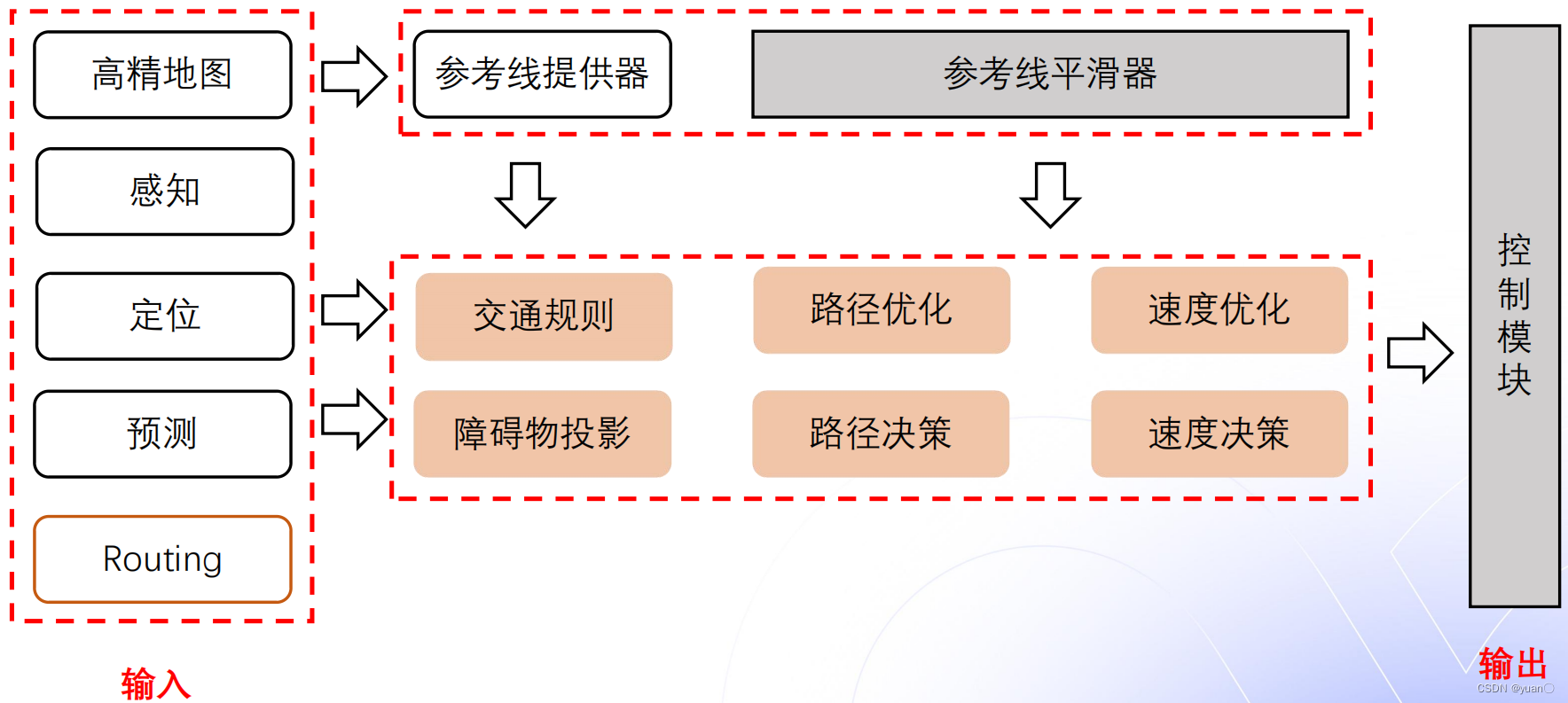
1.1 参考线的作用
1.2 导航规划的路线
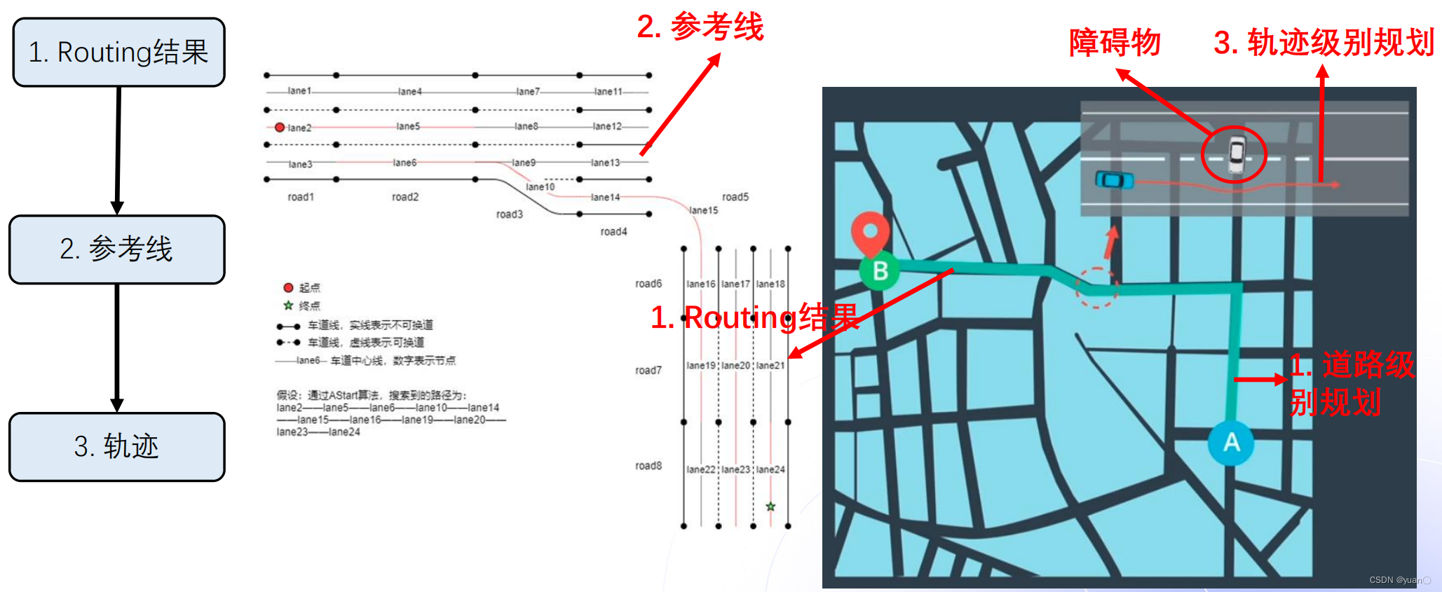 导航规划的路线一般由三个部分组成:Routing、参考线以及轨迹。
Routing: 全局路径规划的结果,一般规划出来的长度为几十公里甚至上百公里,若没有障碍物,车辆将会沿着这条路径一直行驶。若有障碍物,则会由Planning模块发布回Routing模块进行重新规划。
参考线: 决策规划模块根据车辆的实时位置进行计算。参考线的计算依赖于Routing的结果,但同时需要车辆周围的动态信息(障碍物、交通规则)。参考线相当于Routing结果里局部数据(车辆当前位置的一段Routing),距离通常只有几百米。参考线可能会有多条。
轨迹: 是规划决策模块的最终输出结果。轨迹的输入是参考线。轨迹不仅包含车辆的路径信息,也包括车辆的动态信息(速度、加速度等)。
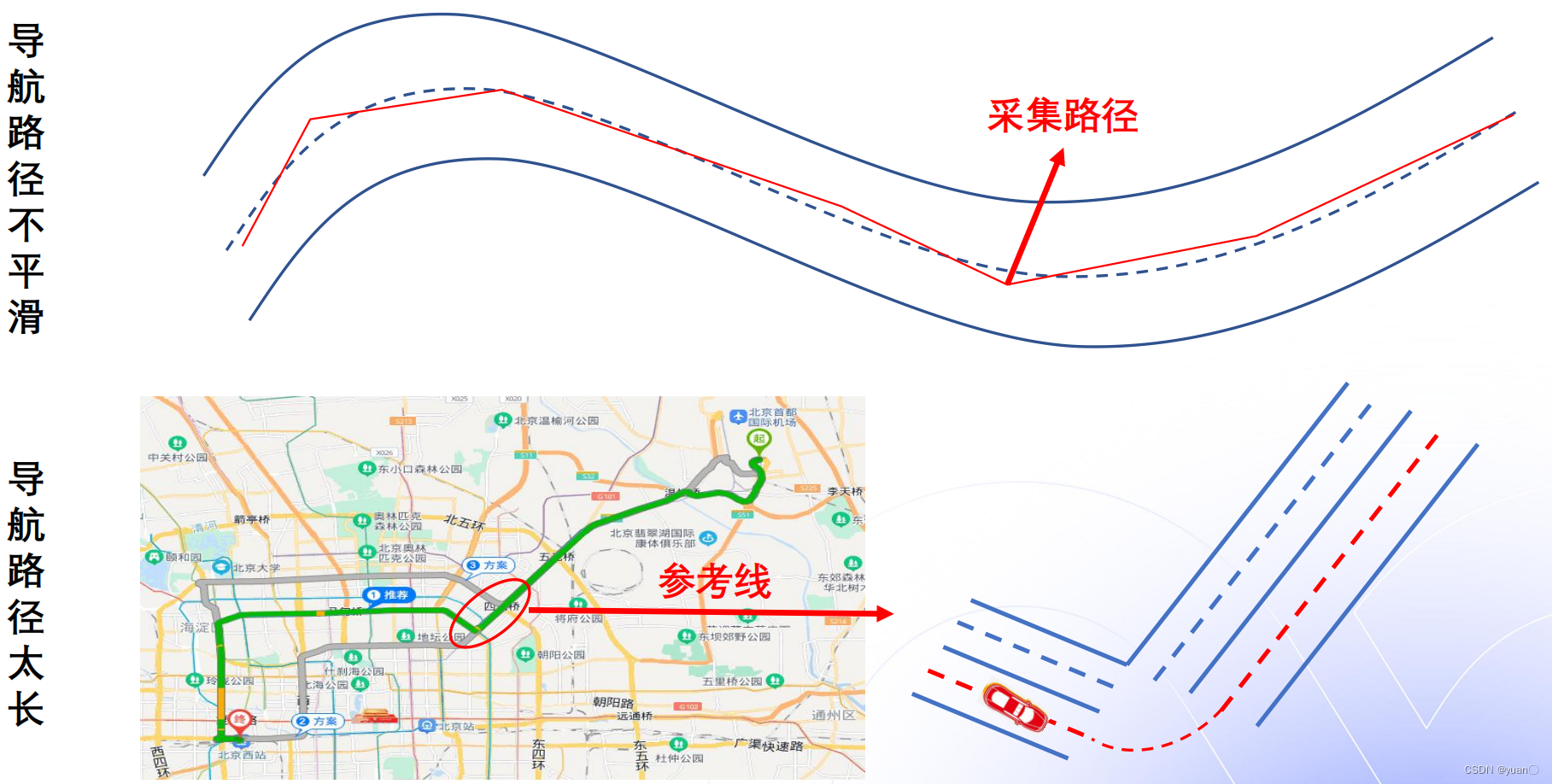
1.3 为什么需要重新生成参考线
1.4 ReferenceLine数据结构
 优先级:当有多条参考线时,具有优先级。
SpeedLimit:车辆在一段参考线里的速度限制。起始点的速度限制/终点的限制
speed_limit_:是一个数组,分段限速。
reference_points_:参考点,同样是数组。
map_path_:地图中的参考线,与planning中的参考线具有一一映射关系,参考点的数目是相同的。
1.5 ReferencePoint数据结构
 ReferencePoint继承自MapPathPoint,MapPathPoint继承自Vec2d。
Vec2d:包含了点的二维数据。
MapPathPoint:包含了点的朝向以及地图上的点对应道路上的点。
ReferencePoint:包含了曲线的曲率与曲率的导数。
1.6 参考线处理流程
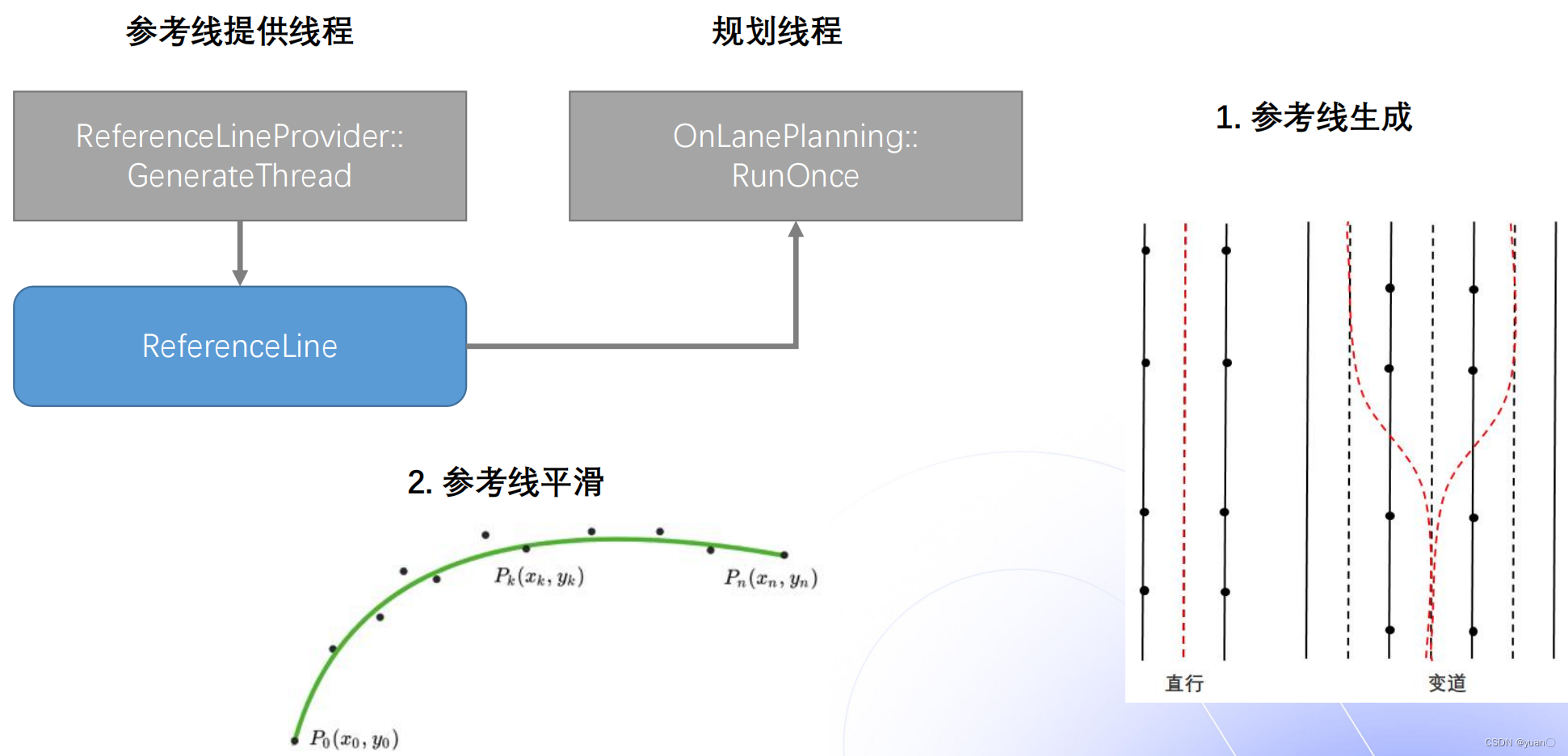 参考线的处理主要涉及两个线程:一个是参考线提供线程,另一个是规划线程。参考线提供线程提供参考线给规划线程去规划出一条轨迹。参考线的处理有两个步骤:首先是参考线的生成,直行时生成一条参考线,当有变道发生时,生成多条参考线。接下来是参考线的平滑,常见的参考线平滑方式有:离散点的平滑(Apollo采用)、螺旋线的平滑以及样条曲线的平滑。
1.7 参考线生成
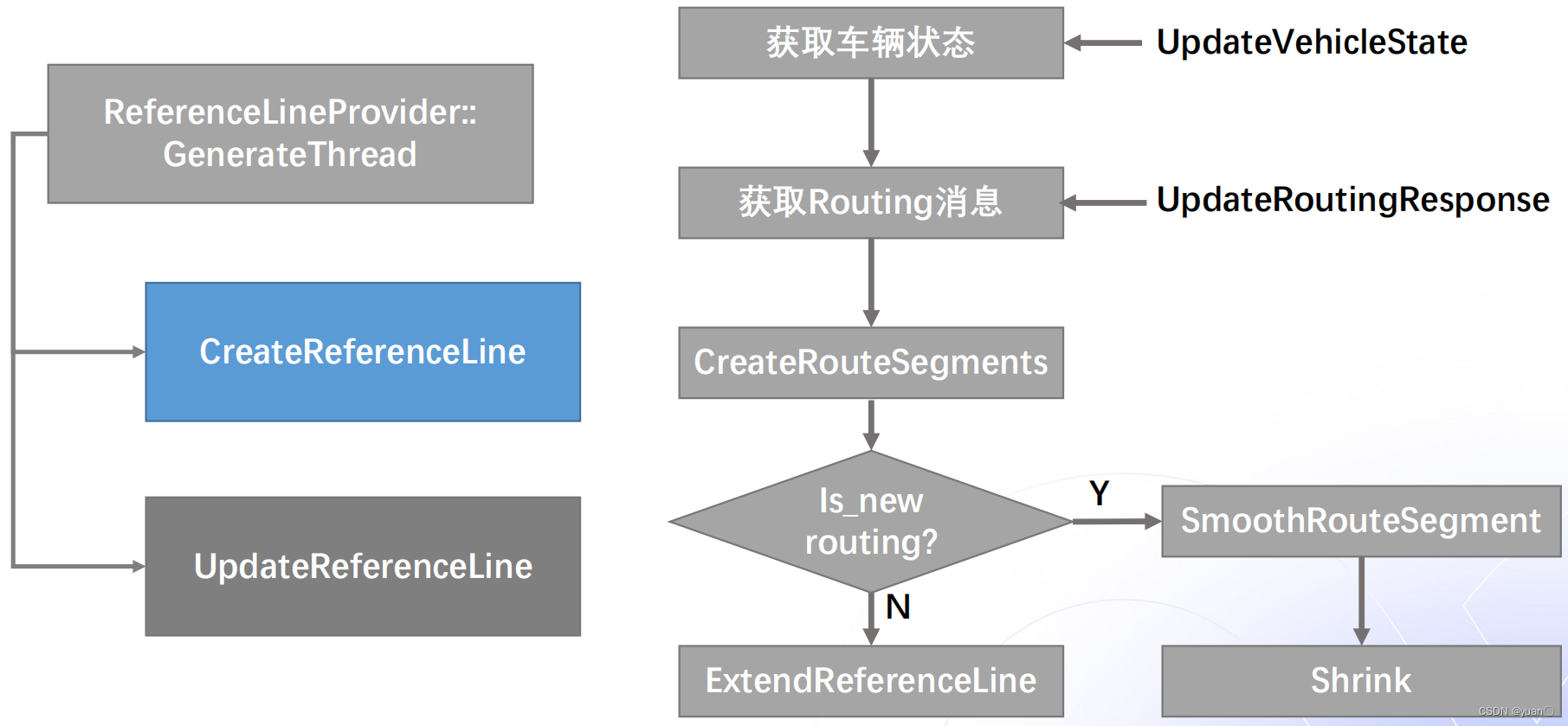 参考线生成是由CreateReferenceLine函数实现的。首先由UpdateVehicleState函数获取车辆的状态,再由UpdateRoutingResponse函数获取Routing的结果,生成RouteSegment。若routing是新生成的,则对其进行平滑与分割;若不是,则沿用上一个周期的参考线,并对其进行扩展与延伸。
2. 参考线平滑算法
2.1 参考线平滑算法总览
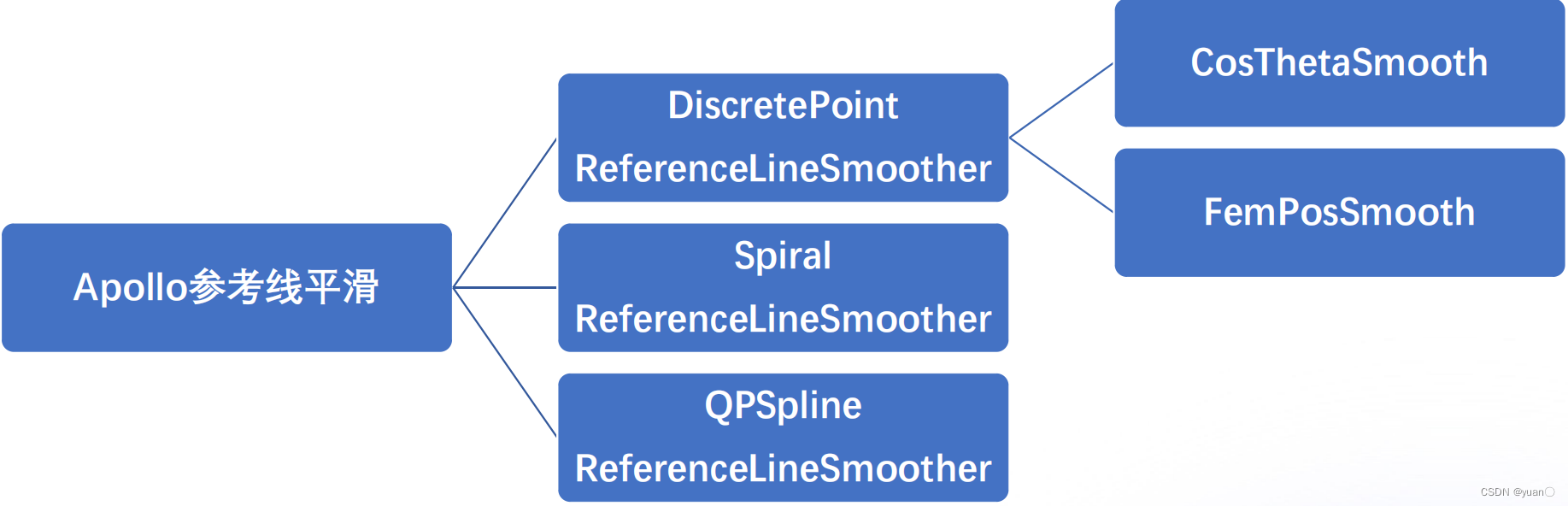 常见的参考线平滑方式有:离散点的平滑(Apollo采用)、螺旋线的平滑以及样条曲线的平滑。
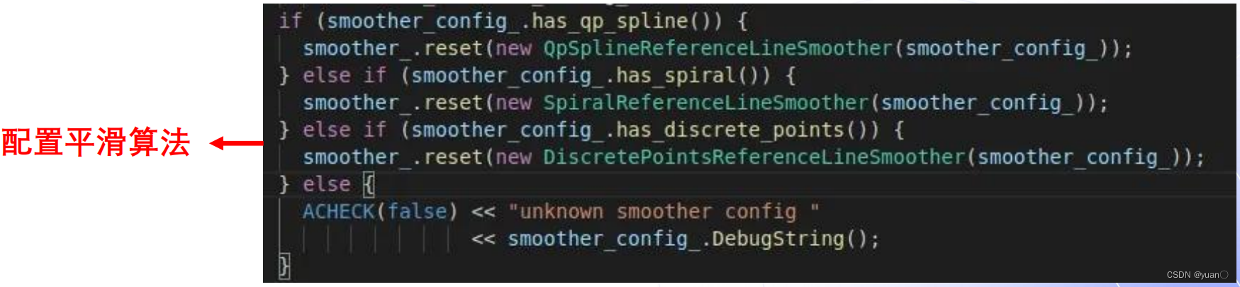
// /home/yuan/apollo-edu/modules/planning/reference_line/reference_line_provider.cc
  if (smoother_config_.has_qp_spline()) {
    smoother_.reset(new QpSplineReferenceLineSmoother(smoother_config_));
  } else if (smoother_config_.has_spiral()) {
    smoother_.reset(new SpiralReferenceLineSmoother(smoother_config_));
  } else if (smoother_config_.has_discrete_points()) {
    smoother_.reset(new DiscretePointsReferenceLineSmoother(smoother_config_));
  } else {
    ACHECK(false) << "unknown smoother config "
                  << smoother_config_.DebugString();
  }
2.2 参考线平滑算法流程
// /home/yuan/apollo-edu/modules/planning/reference_line/reference_line_provider.cc
bool ReferenceLineProvider::SmoothReferenceLine(
    const ReferenceLine &raw_reference_line, ReferenceLine *reference_line) {
  if (!FLAGS_enable_smooth_reference_line) {
    *reference_line = raw_reference_line;
    return true;
  }
  // generate anchor points:
  std::vector<AnchorPoint> anchor_points;
  GetAnchorPoints(raw_reference_line, &anchor_points);
  smoother_->SetAnchorPoints(anchor_points);
  if (!smoother_->Smooth(raw_reference_line, reference_line)) {
    AERROR << "Failed to smooth reference line with anchor points";
    return false;
  }
  if (!IsReferenceLineSmoothValid(raw_reference_line, *reference_line)) {
    AERROR << "The smoothed reference line error is too large";
    return false;
  }
  return true;
}

GetAnchorPoints(raw_reference_line, &anchor_points);用于设置设置中间点
if (!smoother_->Smooth(raw_reference_line, reference_line)) {为平滑算法
2.2.1 设置中间点anchor points
// /home/yuan/apollo-edu/modules/planning/reference_line/reference_line_smoother.h
struct AnchorPoint {
  common::PathPoint path_point;
  double lateral_bound = 0.0;
  double longitudinal_bound = 0.0;
  // enforce smoother to strictly follow this reference point
  bool enforced = false;
};
根据ReferenceLine选取中间点。根据ReferenceLine s(纵向距离上的投影)的值,进行均匀采样,采样的间隔约为0.25m。采样之后得到一系列的AnchorPoint,每个AnchorPoint包含PathPoint、横纵向的裕度以及是否为强约束的判断(若是,则必须为满足横纵向裕度,一条参考线只有首尾的点是强约束)。
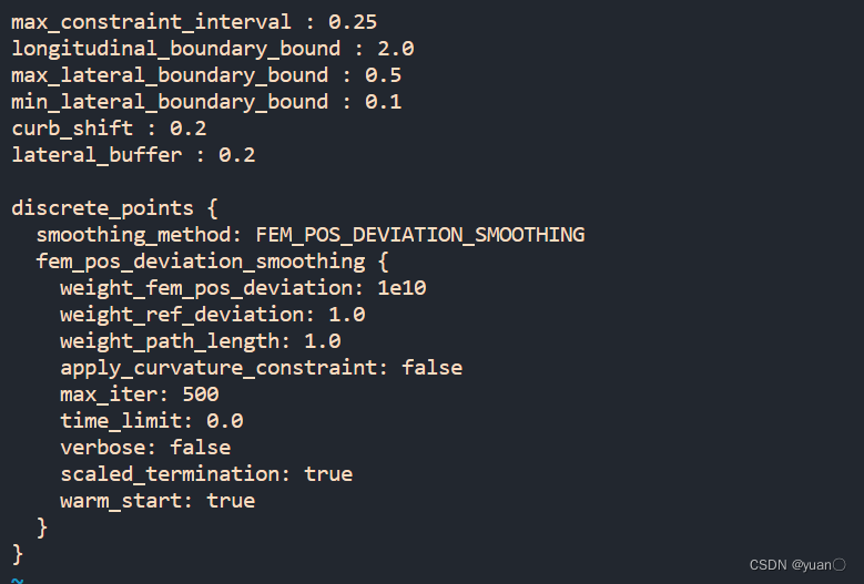
// /home/yuan/apollo-edu/modules/planning/conf/discrete_points_smoother_config.pb.txt
max_constraint_interval : 0.25
longitudinal_boundary_bound : 2.0
max_lateral_boundary_bound : 0.5
min_lateral_boundary_bound : 0.1
curb_shift : 0.2
lateral_buffer : 0.2

discrete_points {
  smoothing_method: FEM_POS_DEVIATION_SMOOTHING
  fem_pos_deviation_smoothing {
    weight_fem_pos_deviation: 1e10
    weight_ref_deviation: 1.0
    weight_path_length: 1.0
    apply_curvature_constraint: false
    max_iter: 500
    time_limit: 0.0
    verbose: false
    scaled_termination: true
    warm_start: true
  }
}
主要参数
max_constraint_interval采样间隔
longitudinal_boundary_bound纵向边界
max_lateral_boundary_bound最大横向边界
min_lateral_boundary_bound最小横向边界
curb_shift与道路边缘的缓冲,若为实线,再增加一个buffer缓冲
lateral_buffer与道路边缘的缓冲
smoothing_method: FEM_POS_DEVIATION_SMOOTHING采用FemPosSmooth平滑算法
weight_fem_pos_deviation平滑度的代价权值
c
o
s
t
s
m
o
o
t
h
{cost_{smooth}}
costsmooth
weight_ref_deviation相对原始点偏移量的代价权值
c
o
s
t
e
r
r
{cost_{err}}
costerr
weight_path_length参考线长度的代价权值
c
o
s
t
l
e
n
g
t
h
{cost_{length}}
costlength
实验时主要考虑平滑,所以将平滑度的权值设得非常大,而其他权值忽略不计。
2.2.2 Smooth函数
/home/yuan/apollo-edu/modules/planning/reference_line/discrete_points_reference_line_smoother.cc
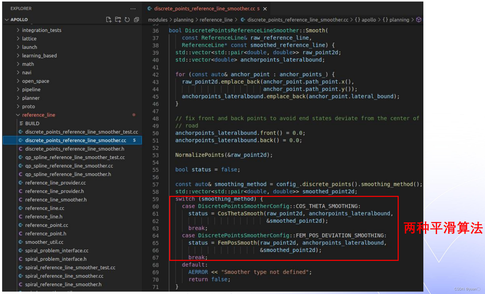 两种平滑算法通过配置文件去选择。
2.2.3FemPosSmooth
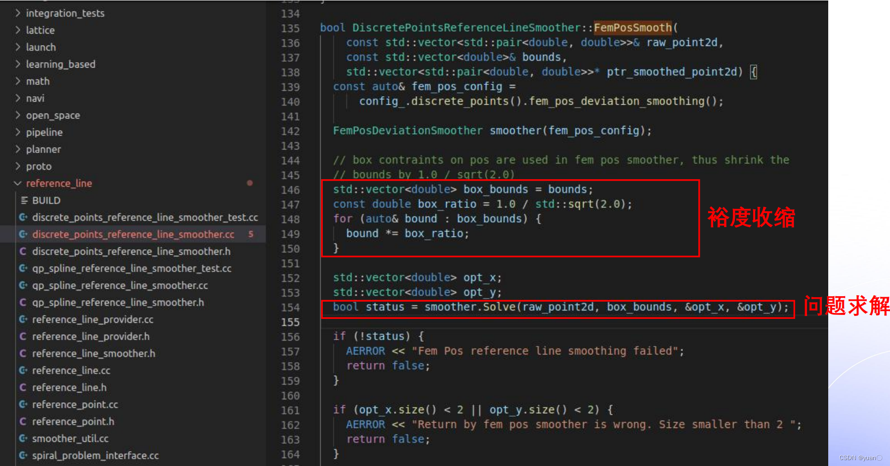
2.2.4 Solve函数
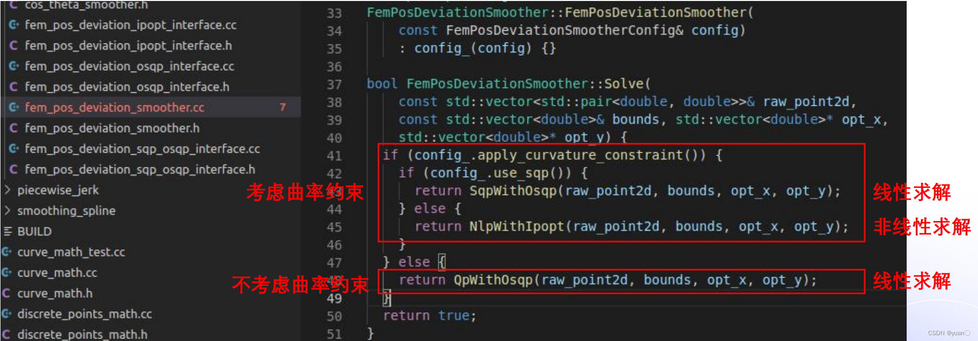
Apollo默认不考虑曲率的约束
2.3 优化问题构造和求解
 Apollo主要是对离散点进行求解,通过构造二次规划问题,利用OSQP求解器进行求解。
优化变量:离散点 P k ( x k , y k ) {P_k(x_k,y_k)} Pk(xk,yk)
优化目标: 平滑度、长度 、相对原始点偏移量
优化函数: c o s t = c o s t s m o o t h + c o s t l e n g t h + c o s t e r r {cost=cost_{smooth}+cost_{length}+cost_{err}} cost=costsmooth+costlength+costerr
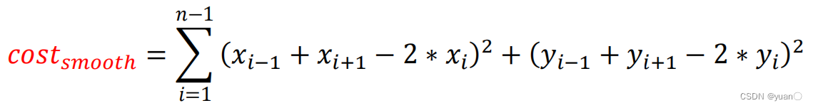
c o s t s m o o t h {cost_{smooth}} costsmooth——平滑度的代价
c o s t l e n g t h {cost_{length}} costlength——参考线长度的代价 c o s t l e n g t h = ∑ i = 0 n − 1 ( x i − x i − 1 ) 2 + ( y i − y i − 1 ) 2 cos{t_{length}} = \sum\limits_{i = 0}^{n - 1} {{{({x_i} - {x_{i - 1}})}^2}} + {({y_i} - {y_{i - 1}})^2} costlength=i=0∑n−1(xi−xi−1)2+(yi−yi−1)2 c o s t e r r {cost_{err}} costerr——相对原始点偏移量的代价 c o s t e r r = ∑ i = 0 n − 1 ( x i − x i _ r e f ) 2 + ( y i − y i _ r e f ) 2 cos{t_{err}} = \sum\limits_{i = 0}^{n - 1} {{{({x_i} - {x_{i\_ref}})}^2}} + {({y_i} - {y_{i\_ref}})^2} costerr=i=0∑n−1(xi−xi_ref)2+(yi−yi_ref)2
2.4 平滑代价
c
o
s
t
s
m
o
o
t
h
{cost_{smooth}}
costsmooth有两种计算方式:FemPosSmooth与CosThetaSmooth。
FemPosSmooth:
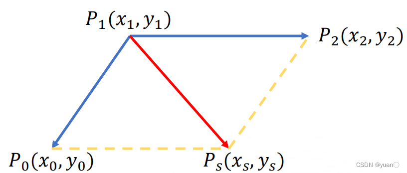
构造方式:一个参考点 P 1 ( x 1 , y 1 ) {P_1(x_1,y_1)} P1(x1,y1)以及其前后两个相邻点 P 0 ( x 0 , y 0 ) {P_0(x_0,y_0)} P0(x0,y0)、 P 2 ( x 2 , y 2 ) {P_2(x_2,y_2)} P2(x2,y2)构成的向量 P 1 P 0 → \overrightarrow {{P_{\rm{1}}}{P_{\rm{0}}}} P1P0、 P 1 P 2 → \overrightarrow {{P_{\rm{1}}}{P_{\rm{2}}}} P1P2的合向量 P 1 P s → \overrightarrow {{P_{\rm{1}}}{P_{\rm{s}}}} P1Ps,求其模的平方。
CosThetaSmooth:

 构造方式:利用相邻两个向量
P
0
P
1
→
\overrightarrow {{P_{\rm{0}}}{P_{\rm{1}}}}
P0P1、
P
1
P
2
→
\overrightarrow {{P_{\rm{1}}}{P_{\rm{2}}}}
P1P2的夹角
θ
\theta
θ的余弦值进行构造。
构造方式:利用相邻两个向量
P
0
P
1
→
\overrightarrow {{P_{\rm{0}}}{P_{\rm{1}}}}
P0P1、
P
1
P
2
→
\overrightarrow {{P_{\rm{1}}}{P_{\rm{2}}}}
P1P2的夹角
θ
\theta
θ的余弦值进行构造。
2.5 约束条件
2.5.1 位置约束
 约束方程:
约束方程:
 保证点在boundingbox之内。
2.5.2 曲率约束

曲率约束首先有以下三个假设:

通过三个假设,构造出约束方程:

∆
s
∆s
∆s是采样平均长度,
c
u
r
c
s
t
r
{cur_{cstr}}
curcstr是最大曲率约束.
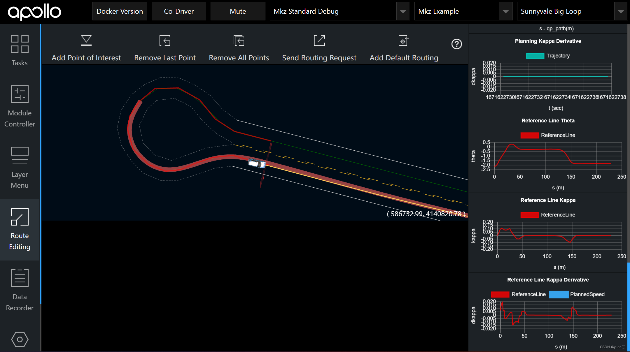
3. U型道路仿真演示
云平台地址——Apollo规划之U型路口仿真调试
启动DreamView
bash scripts/apollo_neo.sh bootstrap
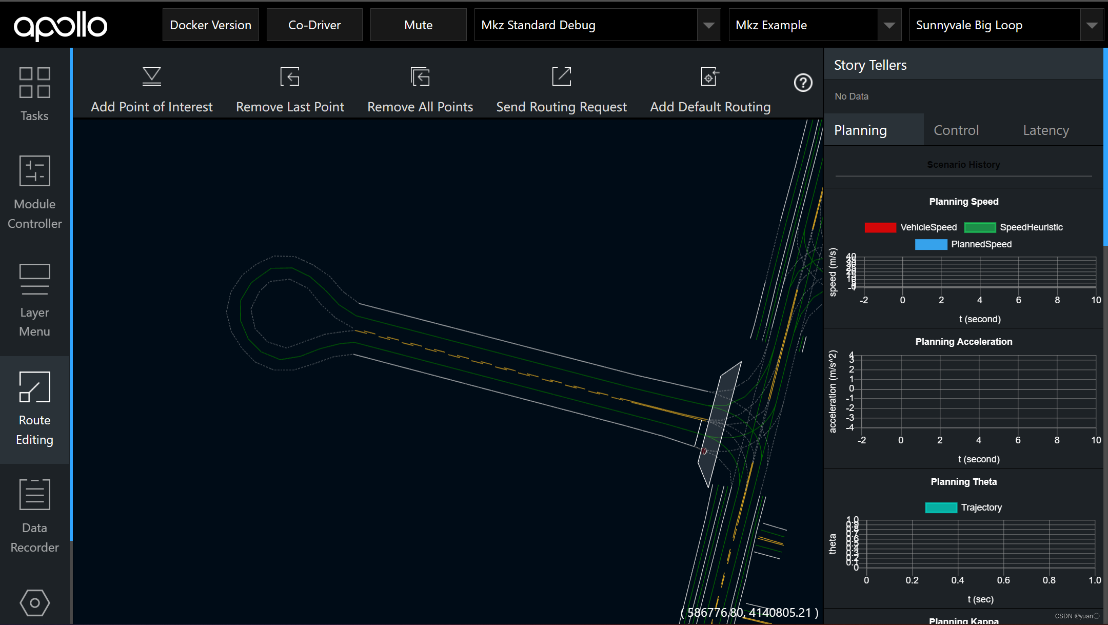
如图所示选好
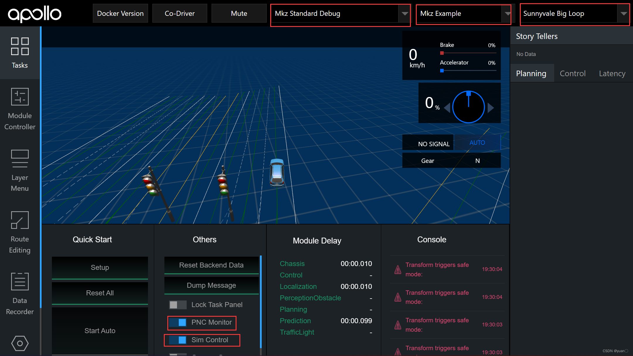

曲率较大的U型弯
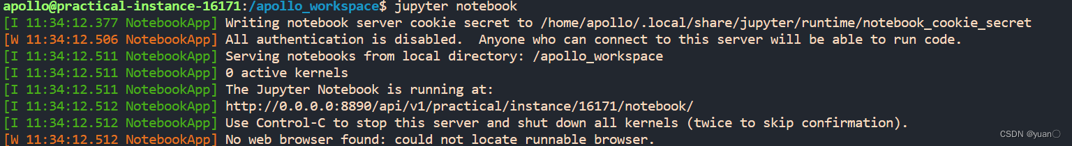
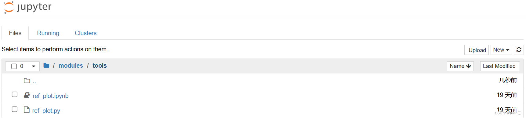
打开 jupyter notebook,绘制脚本在/modules/tools 下
jupyter notebook
脚本代码
import json
import sys
import argparse
import sys
import numpy as np
import matplotlib.pyplot as plt
import math

from cyber.python.cyber_py3.record import RecordReader
from modules.common_msgs.planning_msgs import planning_pb2

class RefLineInfo():
    def __init__(self, x, y, s, theta, kappa, dkappa):
        self.x = x
        self.y = y
        self.s = s
        self.theta = theta
        self.kappa = kappa
        self.dkappa = dkappa

def trim_path_by_distance(adc_trajectory, s):
    path_coords = []
    path_points = adc_trajectory.trajectory_point
    for point in path_points:
        if point.path_point.s <= s:
            path_coords.append([point.path_point.x, point.path_point.y])
    return path_coords

def project(point, ref_line):
    start_point = ref_line[0]
    end_point = start_point
    for line_point in ref_line:
        if line_point.s - ref_line[0].s < 0.2:
            continue
        point_dir = [start_point.x - point.x, start_point.y - point.y]
        line_dir = [line_point.x - start_point.x, line_point.y - start_point.y]
        dot = point_dir[0] * line_dir[0] + point_dir[1] * line_dir[1]
        if dot > 0.0:
            start_point = line_point
            continue
        s = dot / math.sqrt(line_dir[0] * line_dir[0] + line_dir[1] * line_dir[1])
        return start_point.s - s


def align_reference_lines(ref_line1, ref_line2):
    if len(ref_line1) < 2 or len(ref_line2) < 2:
        return [0.0, 0.0]
    if ref_line1[-1].s < 0.5 or ref_line2[-1].s < 0.5:
        return [0.0, 0.0]

    s_ref_line1 = [ref_line1[0].x, ref_line1[0].y]
    cur_index = 1
    e_ref_line1 = [ref_line1[cur_index].x, ref_line1[cur_index].y]
    while ref_line1[cur_index].s < 0.5:
        cur_index = cur_index + 1
        e_ref_line1 = [ref_line1[cur_index].x, ref_line1[cur_index].y]

    start_point2 = ref_line2[0]
    line_dir = [e_ref_line1[0] - s_ref_line1[0], e_ref_line1[1] - s_ref_line1[1]]
    start_dir = [s_ref_line1[0] - start_point2.x, s_ref_line1[1] - start_point2.y]
    dot = line_dir[0] * start_dir[0] + line_dir[1] * start_dir[1]
    if dot > 0.0:
        return [0.0, project(ref_line1[0], ref_line2)]
    return [project(start_point2, ref_line1), 0.0]


def get_ref_line(record_path, ref_line_index=0):
    reader = RecordReader(record_path)
    current_ref_line_index = 0
    for msg in reader.read_messages():
        if msg.topic == "/apollo/planning":
            if current_ref_line_index != ref_line_index:
                current_ref_line_index = current_ref_line_index + 1
                continue
            adc_trajectory = planning_pb2.ADCTrajectory()
            adc_trajectory.ParseFromString(msg.message)

            for path in adc_trajectory.debug.planning_data.path:
                if path.name != 'planning_reference_line':
                    continue
                path_coords = trim_path_by_distance(adc_trajectory, 5.0)

                ref_line = []
                last_theta = path.path_point[0].theta
                for point in path.path_point:
                    if point.theta - last_theta > math.pi:
                        point.theta = point.theta - 2.0 * math.pi
                    elif last_theta - point.theta > math.pi:
                        point.theta = point.theta + 2.0 * math.pi
                    ref_line.append(RefLineInfo(point.x, point.y, point.s, point.theta, point.kappa, point.dkappa))
                return ref_line

def plot_ref_line(start_s, ref_line, use_dot):
    x = []
    y = []
    s = []
    theta = []
    kappa = []
    dkappa = []
    scale_factor = 10.0
    for point in ref_line:
        if point.s < start_s:
            continue
        x.append(point.x)
        y.append(point.y)
        s.append(point.s)
        theta.append(point.theta)
        kappa.append(point.kappa * scale_factor)
        dkappa.append(point.dkappa * scale_factor)
    if use_dot:
        plt.plot(s, theta, 'b--', alpha=0.5, label='theta')
        plt.plot(s, kappa, 'r--', alpha=0.5, label='kappa')
        plt.plot(s, dkappa, 'g--', alpha=0.5, label='dkappa')
    else:
        plt.plot(s, theta, 'b', alpha=0.5, label='theta')
        plt.plot(s, kappa, 'r', alpha=0.5, label='kappa')
        plt.plot(s, dkappa, 'g', alpha=0.5, label='dkappa')

def plot_ref_path(record_file1, record_file2):
    ref_line1 = get_ref_line(record_file1)
    ref_line2 = get_ref_line(record_file2)
    [s1, s2] = align_reference_lines(ref_line1, ref_line2)
    plot_ref_line(s1, ref_line1, True)
    plot_ref_line(s2, ref_line2, False)


record_file1 = './20221221113737.record.00000'
record_file2 = './20221221120201.record.00000'

plot_ref_path(record_file1, record_file2)

plt.legend()
plt.show()
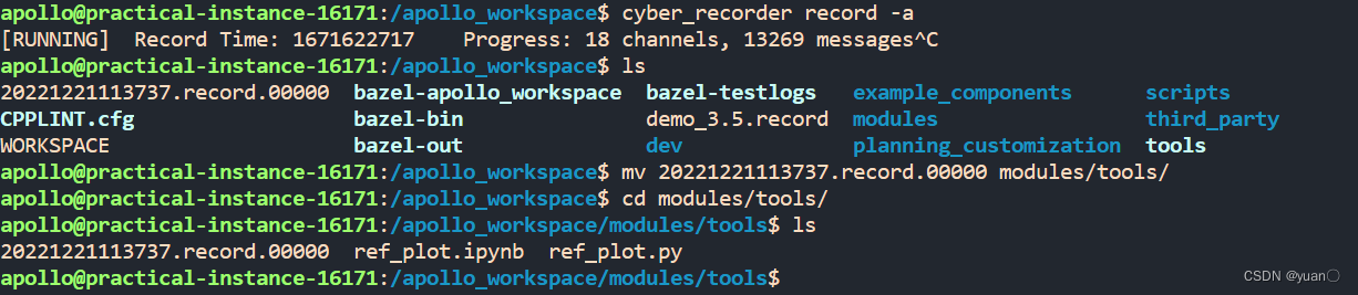
cyber_recorder record -a记录数据
cyber_recorder record -a
我们所需要记录并绘制的数据 将记录好的数据移动到
./modules/tools/下
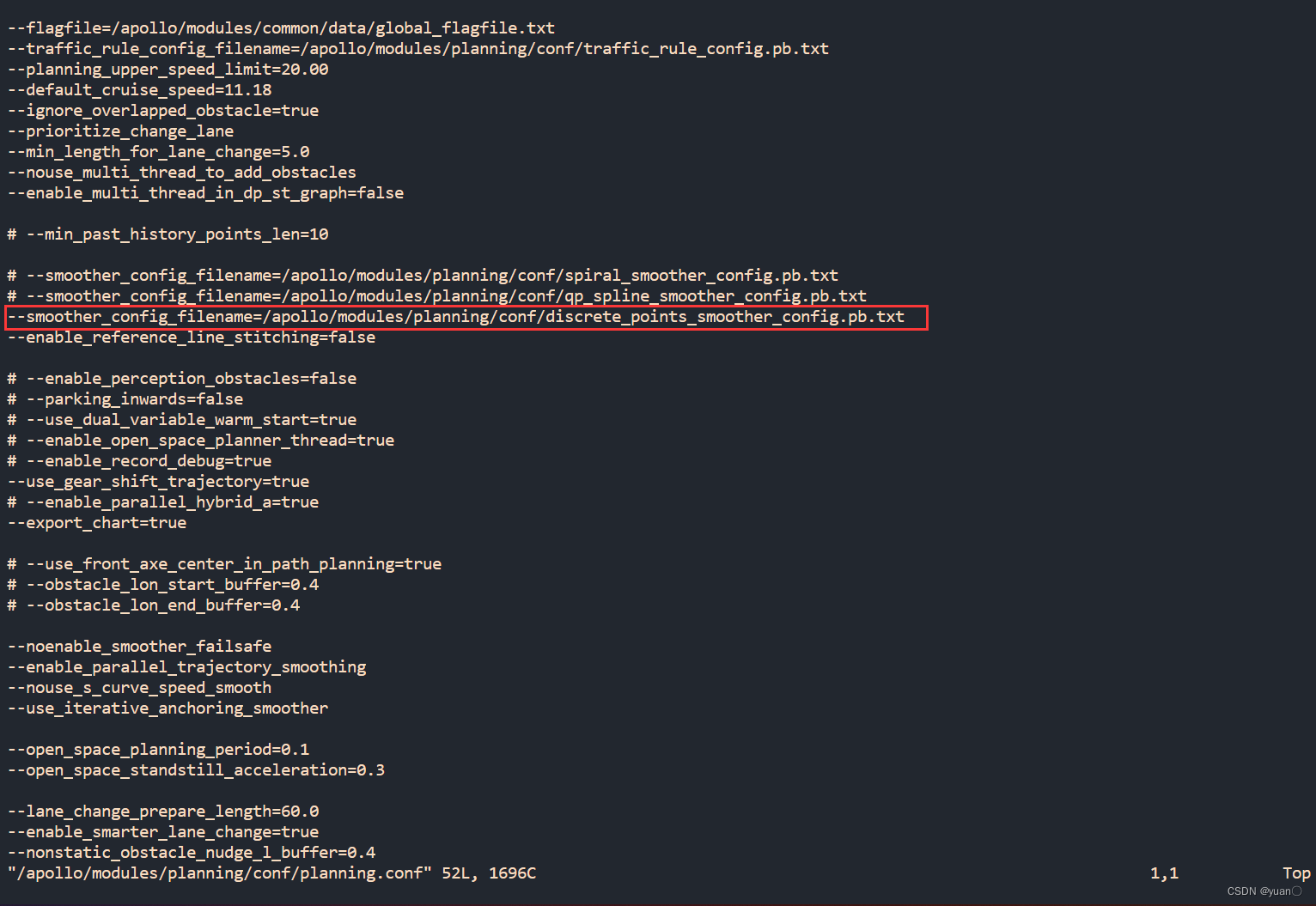
到/apollo/modules/planning/conf/planning.conf 下查看所用的是哪个平滑算法
vim /apollo/modules/planning/conf/planning.conf
进入平滑算法的配置文件
vim /apollo/modules/planning/conf/discrete_points_smoother_config.pb.txt
修改参数,并重启DreamView,防止数据残留。
bash scripts/bootstrap_neo.sh restart
按照之前的步骤得到第二份数据。


max_lateral_boundary_bound : 0.2 其他不变
虚线为未更改的参考线数据,实现为更改后的参考线数据
可以看到,调整横向的参数对整体平滑具有较大的影响。
按照之前的步骤得到第三份数据。

虚线为未更改的参考线数据,实现为更改后的参考线数据
可以看到,调整纵向的参数对于参考线的平滑影响不大。


 1324
1324

 被折叠的 条评论
为什么被折叠?
被折叠的 条评论
为什么被折叠?
 到【灌水乐园】发言


