满足特定分布的互相相关系数为给定值的随机数

事隔两天再看这里写的东西,发现自己的理解偏差太多,这里尤其那些不是转帖来的自己草率写来的内容,仅凭当时一知半解聊作学习笔记自娱自乐而已;如果有人要参考,请务必慎重斟酌,这里的问题和错误我一般不修改. 这里的内容既不能保证反映state-of-the art的进展(比如所谓不能解决的问题可能是有容易的现成的解决方案或集成在某些知名工具里的),提到和分析这些问题的思路或想法也可能是错或漏的,并未有认真的审核.–而且几乎可以肯定这里的说法和理解是有问题的, 是为免责声明

问题

假设在$(0,1)$上均匀分布的随机数发生器已经有了,这个也是最简单的吧. 现在要生成满足$(a,b)$上均匀分布的随机数,以及和它相关系数为$0<s<1$的均值为$\mu$标准差 $\sigma$的正太分布的随机数怎么办?

这里的内容主要是说明了，网上搜来的方法是有局限性的。但是，哪种解决方案才能完美解决问题，并没有说到点子上。

问题的分解

先看看生成相关系数给定的不独立、但同均匀分布的随机数的一般做法是什么：这个是我用英文必应找到的 ; 下面的方法一般只保证相关系数的近似值,并不保证特定分布

Generating Correlated Random Numbers

This article describes common methods that are used in generating correlated random numbers.

1: Generating two sequences of correlated random numbers

Generating two sequences of random numbers with a given correlation is done in two simple steps:

Generate two sequences of uncorrelated normal distributed random numbers $X_1, X_2$

Define a new sequence $Y_1 = \rho X_1 + \sqrt{1-\rho^2} X_2$
This new $Y_1$ sequence will have a
correlation of $\rho$ with the $X_1$ sequence.

Figures: Before and after correlating

Fig.1 Uncorrelated Normal distributed random numbers.

Fig.2 Correlated normal distributed random numbers with a correlatation of 0.80

2: Generating multiple (more than two) sequences of correlated random variables

A general way to generate correlated (normal distributed) random
numbers -with a given correlation matrix C– is done
by finding a matrix U such that

(1)

$$\begin{equation*} U^T U = C \end{equation*}$$

Using this matrix, one can generate correlated random
numbers $R_c$ from uncorrelated
numbers $R$ by multiplying them with this matrix.

(2)

$$\begin{equation*} R_c = R U \end{equation*}$$

There are multiple way to find such a matrix. The two most common methods are

A Cholesky decomposition of the correlation matrix
An Eigenvector decomposition of the correlation matrix (also known as a spectral decomposition)
Example using a Cholesky decomposition

We want to generate random numbers for three variables with the following correlations matrix:

(3)

$$\begin{equation*} C=\begin{bmatrix} 1 & 0.6 & 0.3 \\ 0.6 & 1 & 0.5 \\ 0.3 & 0.5& 1 \end{bmatrix} \end{equation*}$$

Doing a Cholesky decomposition on the correlation matrix give the following matrix:

Function CHOL(matrix As Range)

Dim i As Integer, j As Integer, k As Integer, N As Integer
Dim a() As Double 'the original matrix
Dim element As Double
Dim L_Lower() As Double

N = matrix.Columns.Count

ReDim a(1 To N, 1 To N)
ReDim L_Lower(1 To N, 1 To N)

For i = 1 To N
    For j = 1 To N
        a(i, j) = matrix(i, j).Value
        L_Lower(i, j) = 0
    Next j
Next i

For i = 1 To N
    For j = 1 To N
        element = a(i, j)
        For k = 1 To i - 1
            element = element - L_Lower(i, k) * L_Lower(j, k)
        Next k
        If i = j Then
            L_Lower(i, i) = Sqr(element)
        ElseIf i < j Then
            L_Lower(j, i) = element / L_Lower(i, i)
        End If
    Next j
Next i

CHOL = Application.WorksheetFunction.Transpose(L_Lower)

End Function

(4)

$$\begin{equation*} U=\begin{bmatrix} 1 & 0.6 & 0.3 \\ 0 & 0.8 & 0.4 \\ 0 & 0 & 0.866 \end{bmatrix} \end{equation*}$$

Depending on the algorithm used for the Cholesky decomposition, you can also get the transposed of this matrix. This does doesn’t matter.

We can now transform three uncorrelated random numbers

(5)

$$\begin{equation*} R=\begin{bmatrix} -0.3999 & -1.6041 & -1.0106 \end{bmatrix} \end{equation*}$$

into correlated numbers $R_c$ by multiplying them with the U matrix.

(6) $\begin{equation*} R_c = R U \end{equation*}$

(7)

$$\begin{equation*} = \begin{bmatrix} -0.3999 & -1.6041 & -1.0106 \end{bmatrix} \begin{bmatrix} 1 & 0.6 & 0.3 \\ 0 & 0.8 & 0.4 \\ 0 & 0 & 0.866 \end{bmatrix} \end{equation*}$$

(8)

$$\begin{equation*} = \begin{bmatrix} -0.3999 & -1.5232 & -1.6368 \end{bmatrix} \end{equation*}$$

Example using a Eigenvector decomposition (also known as Spectral Decomposition)

The correlation matrix C has the following eigenvectors

(9)

$$\begin{equation*} E_1=\begin{bmatrix}0.5700\\ 0.6372\\ 0.5188\end{bmatrix}, E_2=\begin{bmatrix}0.6091\\ 0.0960\\ -0.7872\end{bmatrix}, E_3=\begin{bmatrix}0.5515\\ -0.7647\\ 0.3334\end{bmatrix} \end{equation*}$$

and eigenvalues

(10)

$$\begin{equation*} \lambda_1=1.9439, \lambda_2=0.7069, \lambda_3=0.3493 \end{equation*}$$

If we define

(11)

$$\begin{equation*} V= E_i \text{diag}( \sqrt{ \lambda_i}) \end{equation*}$$

(12)

$$\begin{equation*} = \begin{bmatrix} 0.5700 & 0.6091 & 0.5515 \\ 0.6372 & 0.0960 & -0.7647 \\ 0.5188 & -0.7872 & 0.3334 \end{bmatrix} \begin{bmatrix} 1.3942 & 0 & 0 \\ 0 & 0.8402 & 0 \\ 0 & & 0.5911 \end{bmatrix} \end{equation*}$$

(13)

$$\begin{equation*} = \begin{bmatrix} 0.7947 & 0.5121 & 0.3259 \\ 0.8884 & 0.0808 & -0.4520 \\ 0.7232 & -0.6619 & 0.1970 \end{bmatrix} \end{equation*}$$

we get a matrix V that has the property

(14)

$$\begin{equation*} V V^T = C \end{equation*}$$

which gives us the final result for the decomposition

(15)

$$\begin{equation*} U^T U = C, U=V^T \end{equation*}$$

We can now transform three uncorrelated random numbers

(16)

$$\begin{equation*} R=\begin{bmatrix} -0.3999 & -1.6041 & -1.0106 \end{bmatrix} \end{equation*}$$

into correlated numbers R_c by multiplying them with the U matrix.

$$R_c = R U$$

(17)

$$\begin{equation*} = \begin{bmatrix} -0.3999 & -1.6041 & -1.0106 \end{bmatrix} \begin{bmatrix} 0.7947 & 0.8884 & 0.7232 \\ 0.5121 & 0.0808 & -0.6619 \\ 0.7232 & -0.4520 & 0.1970 \end{bmatrix} \end{equation*}$$

(18) $\begin{equation*} = \begin{bmatrix} -1.4687 & -0.0280 & 0.5734 \end{bmatrix} \end{equation*}$

Example Matlab code
The matlab code below decomposes the correlation matrix C into an
upper matrix U using a Cholesky decomposition. Next 10 vectors
with 3 random normal numbers are multiplied with the upper matrix to
generate 10 correlated draws.

上面的是标准方法, 其它网页也容易找到类似介绍,不过英文容易找, 中文太困难了,比如(http://numericalexpert.com/blog/correlated_random_variables/), 不知道是什么原因.

再看看两个均匀或正态随机变量相加之后会得到何种分布,尤其是推导和证明的方法:

两个独立同分布随机变量之和的分布

正态的情况
维基百科: Sum of normally distributed random variables; 涉及特征函数

均匀分布的情况:
两个独立的同0,1均匀分布的随机变量之和服从三角分布的证明

由此可见, 一个正态和一个均匀分布相加, 新的随机变量服从的将会不知道是什么分布。【至少推导是挺繁琐的，结果的解析形式不见得能表示成初等函数形式, 也许从特征函数出发比较方便,不过两个随机变量独立时候的卷积方法应该最好】

回到原始问题：

原始问题工作量

原始问题相当于，需要找到一个服从某个特殊的分布的随机变量 $Z$ , 它跟均匀分布的随机变量 $X$按照相关系数的 $\rho$和$\sqrt{1-\rho^2}$方式加权之和的新随机变量$Y\equiv \rho X+\sqrt{1-\rho^2} Z$ 服从均值为 $\mu$ fang差$\sigma$的正态分布.

等我有空再推导吧.

假设一个连续随机变量$X$服从$[0,1]$上的均匀分布,另一个独立的随机变量$Y$服从标准正态分布, 它们的和$Z=X+Y$的分布密度函数如何?

独立的连续随机变量之和, 新密度函数是老的密度函数的卷积(这个在一般的讲概率的教材中涉及连续随机变量的变换的部分都会讲到,中文英文都有;Schaum’s outline of probability and statistics 3rd Ed)有提到.

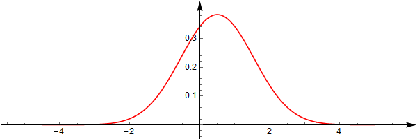
$X$的密度函数:

$$f_X(x)=\left\{\quad \begin{array}{ll} 0 &x<0 \\ 1 & 0\le x \le 1\\ 0&x>1 \end{array} \right.$$

$Y$的密度函数

$$f_Y(x)=\dfrac{1}{\sqrt{2 \pi }}e^{-\dfrac{x^2}{2}},\quad\forall x\in \mathbb R$$

它们的和 $Z=X+Y$ 密度函数 $f_Z(z)$ 相当于两者密度函数的卷积:

$$f_Z(z)=\int_{-\infty}^{+\infty}f_X(x)f_Y(z-x){\rm{d}}x=\int_{0}^{1}f_Y(z-x){\rm{d}}x=\int_{0}^{1}\dfrac{1}{\sqrt{2 \pi }}e^{-\dfrac{(z-x)^2}{2}}{\rm{d}}x$$

这个积分没有办法用初等函数表示,但是可以画出来,看上去很漂亮.

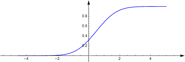
分布函数也无法用初等函数表示

在一起在一起:

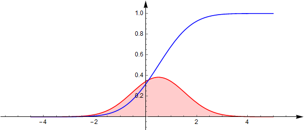
要想得到服从该分布的随机数,在0-1均匀分布随机数的基础上,还需要该分布分布函数的反函数,这可咋办? 除了用迭代之类的数值方法,似乎没有更好办法,好在分布函数单调递增而且光滑。

要想从一个0-1均匀分布和一个未知分布的两个连续随机变量的指定权值的加权和得到一个新的连续随机变量，并使其服从标准正态分布，需要根据权值，先求未知分布的分布函数的反函数。——为什么网上搜到的方法都忽略这一点？

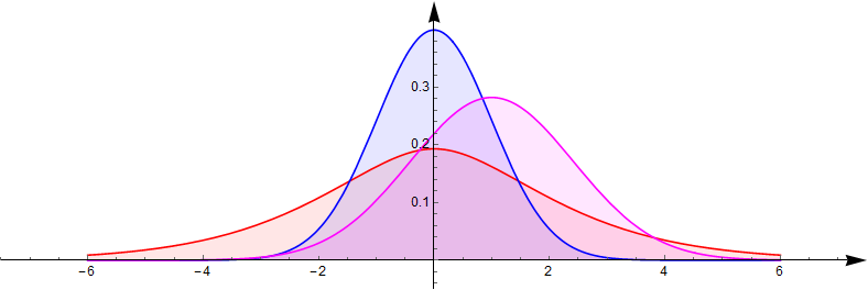
两个相互独立的连续随机变量的标量值函数所服从的新的分布密度函数，也可以构造$\mathbb{R}^2\to\mathbb{R}^2$向量值函数的方式、通过联合分布密度和雅可比行列式的绝对值之积，求新的联合分布函数的边缘分布密度的办法来计算。——大部分情况下恐怕只能计算数值结果，解析结果一般不易用初等函数形式表示。下面是两个独立的标准正态分布(蓝色）变量的积的分布（红色）以及它们的和的分布（紫色）密度的对比。

此外，对于喜欢追求完美的人来说，这里的“去相关变换”显得格外有意义。看上去，这些都是最近的研究成果，难道我无意间看到了一个余温没散的准热点问题？

一种妥协的解决方案

把这个新的分布密度函数跟均值为$\dfrac{1}2$标准差1的正态分布密度作比,发现非常相似:

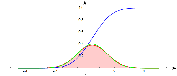
既然随机数都是”伪随机数”,何必在非常近似的分布之间追求严格? 所以实际上调整一下均值之后,问题也就解决了.