


建议通过标题来快速跳转
Vit (Vision Transformer)
Vit把图片打成了patch,然后过标准的TransformerEncoder,最后用CLS token来做分类。关于怎么打成patch再写一些介绍,假设一个图片是224×224×3,每个patch大小是16×16,那么就会有224×224/(16×16)=196的seq_length,每个patch的维度就是16×16×3=768,这个768再过一个Linear层,最终一个图就可以用196×768表示了,再补个cls token,就成了197×768
Vit的位置编码
作者在文中试了几种方式,发现这几种在分类上效果差不多
- 1-dimensional positional embedding
- 2-dimensional positional embedding
- Relative positional embeddings
Vit少了Inductive bias
In CNNs, locality, two-dimensional neighborhood structure, and translation equivariance are baked into each layer throughout the whole model。卷积和FFN相比主要的优先就是局部连接和权值共享。
SwinTransformer
SwinTransformer可以看成是披着ResNet外壳的vision transformer,swin 就是两个关键词:patch + 多尺度。下面结合code来说一些重点的细节:
总览图
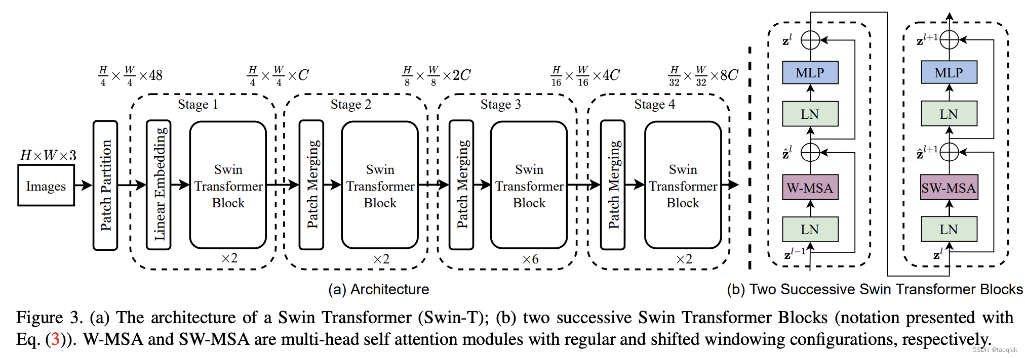
这里W-MSA缩写是window-multi head self attention,SW-MSA缩写是shifted window-multi head self attention。整个模型采取层次化的设计,一共包含4个Stage,每个stage都会缩小输入特征图的分辨率,像CNN一样逐层扩大感受野。
- 在输入开始的时候,做了一个Patch Embedding,将图片切成一个个图块,并嵌入到Embedding。
- 在每个Stage里,由Patch Merging和多个Block组成。其中Patch Merging模块主要在每个Stage一开始降低图片分辨率(把H×W×C转成(H/2)×(W/2)×(2C)),把进而形成层次化的设计,同时也能节省一定运算量。
- 而Block具体结构如右图所示,主要是LayerNorm,MLP,window-multi head self attention和 shifted window-multi head self attention组成。所以一个Block里至少有两个MSA结构
结合代码实现看更多细节
Patch Embedding
在输入进Block前,我们需要将图片切成一个个patch,然后嵌入向量。采用patch_size * patch_size的窗口大小,通过nn.Conv2d,将stride,kernelsize设置为patch_size大小,patch_size设置为4。值得注意的是SwinTransformer的patch_size×patch_size是4×4,而Vit的patch_size×patch_size是16×16,所以SwinTransformer的序列长度就会长很多,这对于Transformer是吃不消的,因此就有了W-MSA放在一个窗口内减少复杂度。
class PatchEmbed(nn.Module):
    def __init__(self,
                 img_size=224,
                 patch_size=4,
                 in_chans=3,
                 embed_dim=96,
                 norm_layer=None):
        super().__init__()
        img_size = to_2tuple(img_size)
        patch_size = to_2tuple(patch_size)
        patches_resolution = [
            img_size[0] // patch_size[0], img_size[1] // patch_size[1]
        ]
        self.img_size = img_size
        self.patch_size = patch_size
        self.patches_resolution = patches_resolution
        self.num_patches = patches_resolution[0] * patches_resolution[1]

        self.in_chans = in_chans
        self.embed_dim = embed_dim

        self.proj = nn.Conv2d(in_chans,
                              embed_dim,
                              kernel_size=patch_size,
                              stride=patch_size)
        if norm_layer is not None:
            self.norm = norm_layer(embed_dim)
        else:
            self.norm = None

    def forward(self, x):
        B, C, H, W = x.shape
        # FIXME look at relaxing size constraints
        assert H == self.img_size[0] and W == self.img_size[1], \
            f"Input image size ({H}*{W}) doesn't match model ({self.img_size[0]}*{self.img_size[1]})."
        x = self.proj(x).flatten(2).transpose(1, 2)  # B Ph*Pw C
        if self.norm is not None:
            x = self.norm(x)
        return x
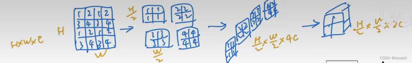
Patch Merging
这一步用Yi Zhu老师的图最好了,Patch Merging模块主要在每个Stage一开始降低图片分辨率(把H×W×C转成(H/2)×(W/2)×(2C)),把进而形成层次化的设计,同时也能节省一定运算量。
class PatchMerging(nn.Module):
    r""" Patch Merging Layer.

    Args:
        input_resolution (tuple[int]): Resolution of input feature.
        dim (int): Number of input channels.
        norm_layer (nn.Module, optional): Normalization layer.  Default: nn.LayerNorm
    """
    def __init__(self, input_resolution, dim, norm_layer=nn.LayerNorm):
        super().__init__()
        self.input_resolution = input_resolution
        self.dim = dim
        self.reduction = nn.Linear(4 * dim, 2 * dim, bias=False)
        self.norm = norm_layer(4 * dim)

    def forward(self, x):
        """
        x: B, H*W, C
        """
        H, W = self.input_resolution
        B, L, C = x.shape
        assert L == H * W, "input feature has wrong size"
        assert H % 2 == 0 and W % 2 == 0, f"x size ({H}*{W}) are not even."

        x = x.view(B, H, W, C)

        x0 = x[:, 0::2, 0::2, :]  # B H/2 W/2 C
        x1 = x[:, 1::2, 0::2, :]  # B H/2 W/2 C
        x2 = x[:, 0::2, 1::2, :]  # B H/2 W/2 C
        x3 = x[:, 1::2, 1::2, :]  # B H/2 W/2 C
        x = torch.cat([x0, x1, x2, x3], -1)  # B H/2 W/2 4*C
        x = x.view(B, -1, 4 * C)  # B H/2*W/2 4*C

        x = self.norm(x)
        x = self.reduction(x)

        return x
Window Attention
这部分关键点就两点:
- 刚才提到的用了Window减少复杂度
- 加了相对位置编码,把 S o f t M a x ( Q K T / d ) SoftMax(QK^T/\sqrt d) SoftMax(QKT/d)变成 S o f t M a x ( ( Q K T + B ) / d ) SoftMax((QK^T+B)/\sqrt d) SoftMax((QKT+B)/d),其中B就是那个相对位置编码
Window Attention复杂度
这里hw分别是图片的高宽,C是embedding dim。Transformer复杂度看了无数遍是
O
(
n
2
d
)
O(n^2d)
O(n2d),其中n是序列长度,也就是这里的hw,d是embedding dim,也就是这里的C。但实际上经常脑子晕搞不起是几倍的
n
2
d
n^2d
n2d,这里结合代码进一步明确下Transformer的复杂度:
- scaled dot production复杂度: 2 n 2 d = 2 ( h w ) 2 C 2n^2d=2(hw)^2C 2n2d=2(hw)2C
- Q、K、V三个矩阵和输出前的dense: 3 n d 2 + n d 2 = 4 n d 2 = 4 h w C 2 3nd^2+nd^2=4nd^2=4hwC^2 3nd2+nd2=4nd2=4hwC2
- position-size feedforward: 4 n d 2 + 4 n d 2 = 8 n d 2 4nd^2+4nd^2=8nd^2 4nd2+4nd2=8nd2,这部分在公式(1)中不需要体现,Swin里没这些
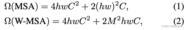
公式(2)和公式(1)相比,M表示window_size,那么有
Ω
(
W
−
M
S
A
)
=
h
M
×
w
M
×
(
4
M
2
C
2
+
2
(
M
2
)
2
C
)
\Omega(W-MSA)=\frac{h}{M}\times\frac{w}{M}\times(4M^2C^2+2(M^2)^2C)
Ω(W−MSA)=Mh×Mw×(4M2C2+2(M2)2C)
对于维度为224 * 224的图片,patch_size=4,window_size=7,h=56, w=56,可以带入公式(1)和公式(2)算一下复杂度,主要是hw被缩到了 M 2 M^2 M2
下面是multi-head attention的一个典型实现:
import torch.nn as nn
import torch
from torch import Tensor
import math

class MyMultiheadAttention(nn.Module):
    def __init__(self, embed_dim, num_heads):
        super(MyMultiheadAttention, self).__init__()
        self.embed_dim = embed_dim
        self.num_heads = num_heads
        self.W_Q = nn.Linear(embed_dim,embed_dim)
        self.W_K = nn.Linear(embed_dim,embed_dim)
        self.W_V = nn.Linear(embed_dim,embed_dim)
        self.fc = nn.Linear(embed_dim,embed_dim)
        self.ln = nn.LayerNorm(embed_dim)

    def scaled_dot_product_attention(self, q:Tensor, k:Tensor, v:Tensor):
        B, Nt, E = q.shape
        q = q / math.sqrt(E)
        # (B, Nt, E) x (B, E, Ns) -> (B, Nt, Ns)
        attn = torch.bmm(q, k.transpose(-2, -1))
        attn = attn.softmax(dim=-1)
        # (B, Nt, Ns) x (B, Ns, E) -> (B, Nt, E)
        output = torch.bmm(attn, v)
        return output,attn

    def forward(self, query:Tensor, key:Tensor, value:Tensor):
        # assert query, key, value have the same shape
        # query shape: tgt_len, bsz, input_embedding
        tgt_len, bsz, embed_dim = query.shape
        head_dim = embed_dim // self.num_heads
        q = self.W_Q(query).reshape(tgt_len, bsz * num_heads, head_dim).transpose(0, 1)
        k = self.W_K(key).reshape(tgt_len, bsz * num_heads, head_dim).transpose(0, 1)
        v = self.W_V(value).reshape(tgt_len, bsz * num_heads, head_dim).transpose(0, 1)
        self_output,attn = self.scaled_dot_product_attention(q, k, v)
        # self_output: bsz * num_heads, tgt_len, head_dim
        # attn: bsz * num_heads, tgt_len, src_len
        output = self.fc(self_output.transpose(0, 1).reshape(tgt_len, bsz, -1))
        # hugging face版把fc放到BertSelfOutput里去了
        return self.ln(output+query),attn

embed_dim,num_heads=100,5
seq_len,bsz = 2,3

multihead_attn = nn.MultiheadAttention(embed_dim, num_heads)
query = torch.ones(seq_len, bsz, embed_dim)
key = torch.ones(seq_len, bsz, embed_dim)
value = torch.ones(seq_len, bsz, embed_dim)

attn_output, attn_output_weights = multihead_attn(query, key, value)
print('attn_output={}'.format(attn_output.shape))
print('attn_output_weights={}'.format(attn_output_weights.shape))
print('--------------')
my_multihead_attn = MyMultiheadAttention(embed_dim, num_heads)
my_attn_output, my_attn_output_weights = my_multihead_attn(query, key, value)
print('my_attn_output={}'.format(attn_output.shape))
print('my_attn_output_weights={}'.format(attn_output_weights.shape))

'''
输出如下:
attn_output=torch.Size([2, 3, 100])
attn_output_weights=torch.Size([3, 2, 2])
--------------
my_attn_output=torch.Size([2, 3, 100])
my_attn_output_weights=torch.Size([3, 2, 2])
'''
下面摘录了实现window attention中的重要代码:
模型在计算window_attention之前,会对输入数据进行partition,进行并行计算,将
(
B
,
h
,
w
,
C
)
(B, h,w, C)
(B,h,w,C)维度的向量,转化为
(
B
∗
h
∗
w
M
∗
M
,
M
,
M
,
C
)
(B*\frac{h*w}{M*M}, M,M, C)
(B∗M∗Mh∗w,M,M,C),其中
M
M
M表示window_size的大小。
def window_partition(x, window_size):
    """
    Args:
        x: (B, H, W, C)
        window_size (int): window size
    Returns:
        windows: (num_windows*B, window_size, window_size, C)
    """
    B, H, W, C = x.shape
    x = x.view(B, H // window_size, window_size, W // window_size, window_size, C)
    windows = x.permute(0, 1, 3, 2, 4, 5).contiguous().view(-1, window_size, window_size, C)
    return windows
完成window_attention之后,会对数据进行reverse,将 ( B ∗ h ∗ w M ∗ M , M , M , C ) (B*\frac{h*w}{M*M}, M,M, C) (B∗M∗Mh∗w,M,M,C)维度的向量,转化为 ( B , h , w , C ) (B, h,w, C) (B,h,w,C):
def window_reverse(windows, window_size, H, W):
    """
    Args:
        windows: (num_windows*B, window_size, window_size, C)
        window_size (int): Window size
        H (int): Height of image
        W (int): Width of image
    Returns:
        x: (B, H, W, C)
    """
    B = windows.shape[0] // (H * W // window_size // window_size)
    x = windows.view(B, H // window_size, W // window_size, window_size, window_size, -1)
    x = x.permute(0, 1, 3, 2, 4, 5).contiguous().view(B, H, W, -1)
    return x
Window attention部分的计算跟传统的attention计算方式基本是一致的:
class WindowAttention(nn.Module):
    r""" Window based multi-head self attention (W-MSA) module with relative position bias.
    It supports both of shifted and non-shifted window.
    """
    def __init__(self,
                 dim,
                 window_size,
                 num_heads,
                 qkv_bias=True,
                 qk_scale=None,
                 attn_drop=0.,
                 proj_drop=0.):
    pass

    def forward(self, x, mask=None):
        """
        Args:
            x: input features with shape of (num_windows*B, N, C)
            mask: (0/-inf) mask with shape of (num_windows, Wh*Ww, Wh*Ww) or None
        """
        B_, N, C = x.shape
        qkv = self.qkv(x).reshape(B_, N, 3, self.num_heads, C // self.num_heads).permute(2, 0, 3, 1, 4)
        q, k, v = qkv[0], qkv[1], qkv[2]  # make torchscript happy (cannot use tensor as tuple)

        q = q * self.scale
        attn = (q @ k.transpose(-2, -1))
        # attention bias相对位置编码
        relative_position_bias = self.relative_position_bias_table[
            self.relative_position_index.view(-1)].view(
                self.window_size[0] * self.window_size[1],
                self.window_size[0] * self.window_size[1],
                -1)  # Wh*Ww,Wh*Ww,nH
        relative_position_bias = relative_position_bias.permute(
            2, 0, 1).contiguous()  # nH, Wh*Ww, Wh*Ww
        attn = attn + relative_position_bias.unsqueeze(0)

        if mask is not None:
            nW = mask.shape[0]
            attn = attn.view(B_ // nW, nW, self.num_heads, N, N) + mask.unsqueeze(1).unsqueeze(0)
            attn = attn.view(-1, self.num_heads, N, N)
            attn = self.softmax(attn)
        else:
            attn = self.softmax(attn)

        attn = self.attn_drop(attn)

        x = (attn @ v).transpose(1, 2).reshape(B_, N, C)
        x = self.proj(x)
        x = self.proj_drop(x)
        return x
其中比较难理解的是"relative_position_index"的计算部分,这块拿出来单独分析。作者是采用了二维坐标来表示windows内各个token的相对位置,相对位置参数表参数量为 ( 2 M − 1 ) ∗ ( 2 M − 1 ) (2M-1)*(2M-1) (2M−1)∗(2M−1)
相对位置编码relative_position_index(比较绕)
#define a parameter table of relative position bias
self.relative_position_bias_table = nn.Parameter(torch.zeros((2 * window_size[0] - 1) * (2 * window_size[1] - 1), num_heads))  # 2*Wh-1 * 2*Ww-1, nH

# get pair-wise relative position index for each token inside the window
coords_h = torch.arange(self.window_size[0])
coords_w = torch.arange(self.window_size[1])
coords = torch.stack(torch.meshgrid([coords_h, coords_w]))  # 2, Wh, Ww
coords_flatten = torch.flatten(coords, 1)  # 2, Wh*Ww
relative_coords = coords_flatten[:, :, None] - coords_flatten[:, None, :]  # 2, Wh*Ww, Wh*Ww
relative_coords = relative_coords.permute(1, 2, 0).contiguous()  # Wh*Ww, Wh*Ww, 2
relative_coords[:, :, 0] += self.window_size[0] - 1  # shift to start from 0
relative_coords[:, :, 1] += self.window_size[1] - 1
relative_coords[:, :, 0] *= 2 * self.window_size[1] - 1
relative_position_index = relative_coords.sum(-1)  # Wh*Ww, Wh*Ww
self.register_buffer("relative_position_index", relative_position_index)
首先QK计算出来的Attention张量形状为(numWindows×B, num_heads, window_size×window_size, window_size×window_size),其中window_size×window_size刚好是序列长度,这不难理解。多头经常会被合并到batch里一起算,numWindows×B×num_heads最后被reshape成numWindows×B,num_heads
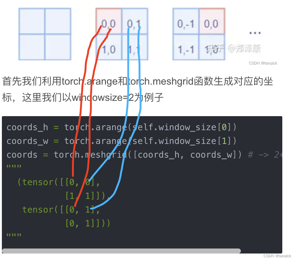
而对于Attention张量来说,以不同元素为原点,其他元素的坐标也是不同的,以window_size=2为例,其相对位置编码如下图所示
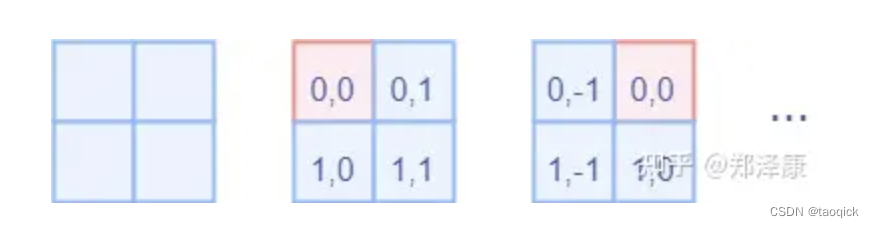
首先我们利用torch.arange和torch.meshgrid函数生成对应的坐标,这里我们以windowsize=2为例子
coords_h = torch.arange(self.window_size[0])
coords_w = torch.arange(self.window_size[1])
coords = torch.meshgrid([coords_h, coords_w]) # -> 2*(wh, ww)
"""
  (tensor([[0, 0],
           [1, 1]]),
   tensor([[0, 1],
           [0, 1]]))
"""
meshgrid输出是一个tuple,tuple中含有2个元素,对应位置的拼在一起就是图示结果:
然后堆叠起来,展开为一个二维向量
coords = torch.stack(coords)  # 2, Wh, Ww
coords_flatten = torch.flatten(coords, 1)  # 2, Wh*Ww
"""
tensor([[0, 0, 1, 1],
        [0, 1, 0, 1]])
"""
利用广播机制,分别在第一维,第二维,插入一个维度,进行广播相减,得到 2, wh×ww, wh×ww的张量
relative_coords_first = coords_flatten[:, :, None]  # 2, wh*ww, 1
relative_coords_second = coords_flatten[:, None, :] # 2, 1, wh*ww
relative_coords = relative_coords_first - relative_coords_second # 最终得到 2, wh*ww, wh*ww 形状的张量
因为采取的是相减,所以得到的索引是从负数开始的,我们加上偏移量,让其从0开始。
relative_coords = relative_coords.permute(1, 2, 0).contiguous() # Wh*Ww, Wh*Ww, 2
relative_coords[:, :, 0] += self.window_size[0] - 1
relative_coords[:, :, 1] += self.window_size[1] - 1
后续我们需要将其展开成一维偏移量。而对于(1,2)和(2,1)这两个坐标。在二维上是不同的,但是通过将x,y坐标相加转换为一维偏移的时候,他的偏移量是相等的。
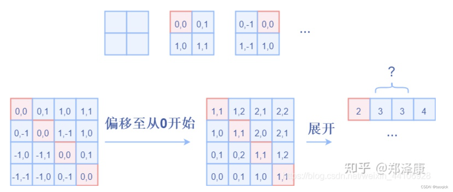
所以最后我们对其中做了个乘法操作,以进行区分
relative_coords[:, :, 0] *= 2 * self.window_size[1] - 1
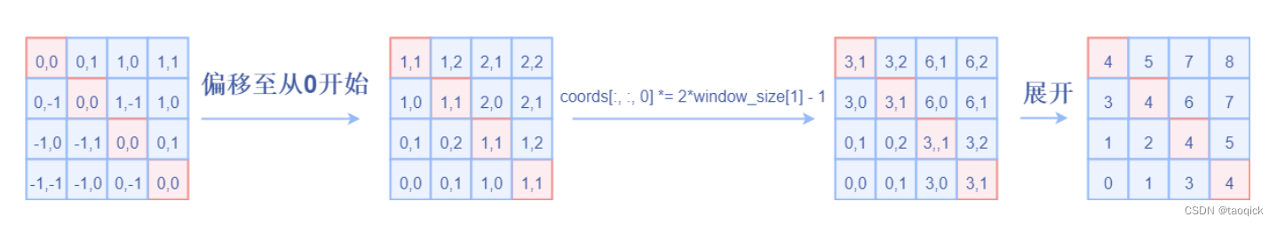
然后再最后一维上进行求和,展开成一个一维坐标,并注册为一个不参与网络学习的变量
relative_position_index = relative_coords.sum(-1)  # Wh*Ww, Wh*Ww
self.register_buffer("relative_position_index", relative_position_index)
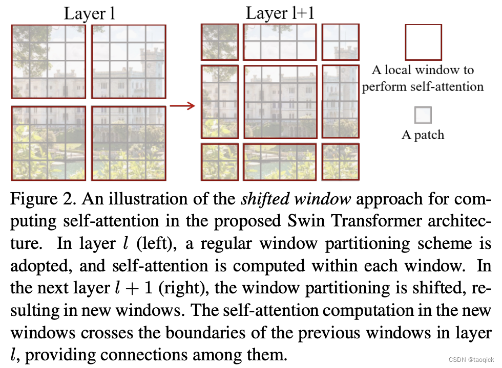
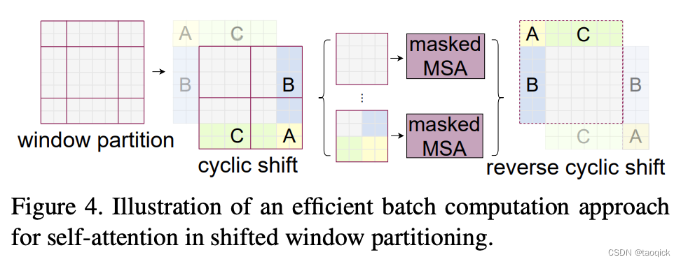
Shifted Window Attention
前面的Window Attention是在每个窗口下计算注意力的,为了更好的和其他window进行信息交互,Swin Transformer还引入了shifted window操作。每次shifted window操作都是一样的,按照window size的一半,向右下方移动。
移动之后,MSA要计算9个,为了节省计算量,进行了拼接。拼接之后计算量变为4。
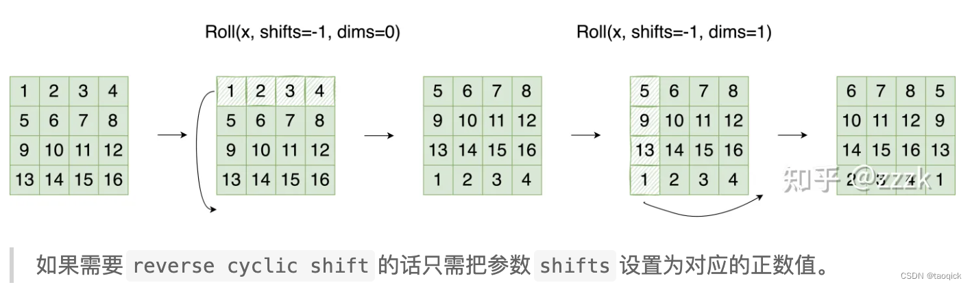
特征图移位操作
代码里对特征图移位是通过torch.roll来实现的,下面是示意图
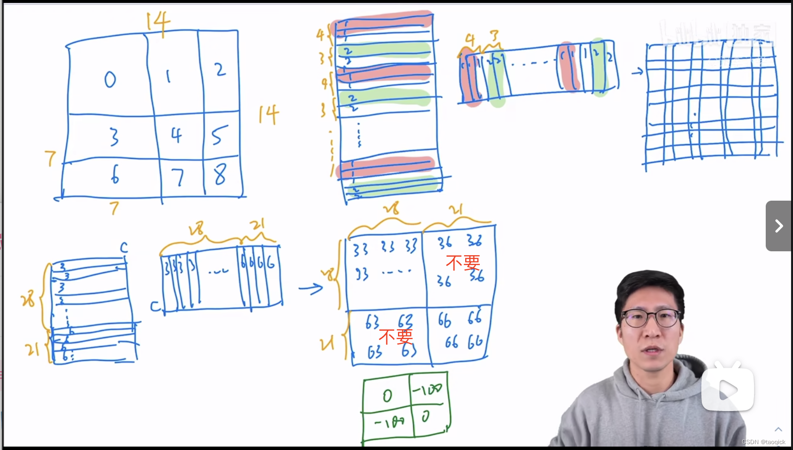
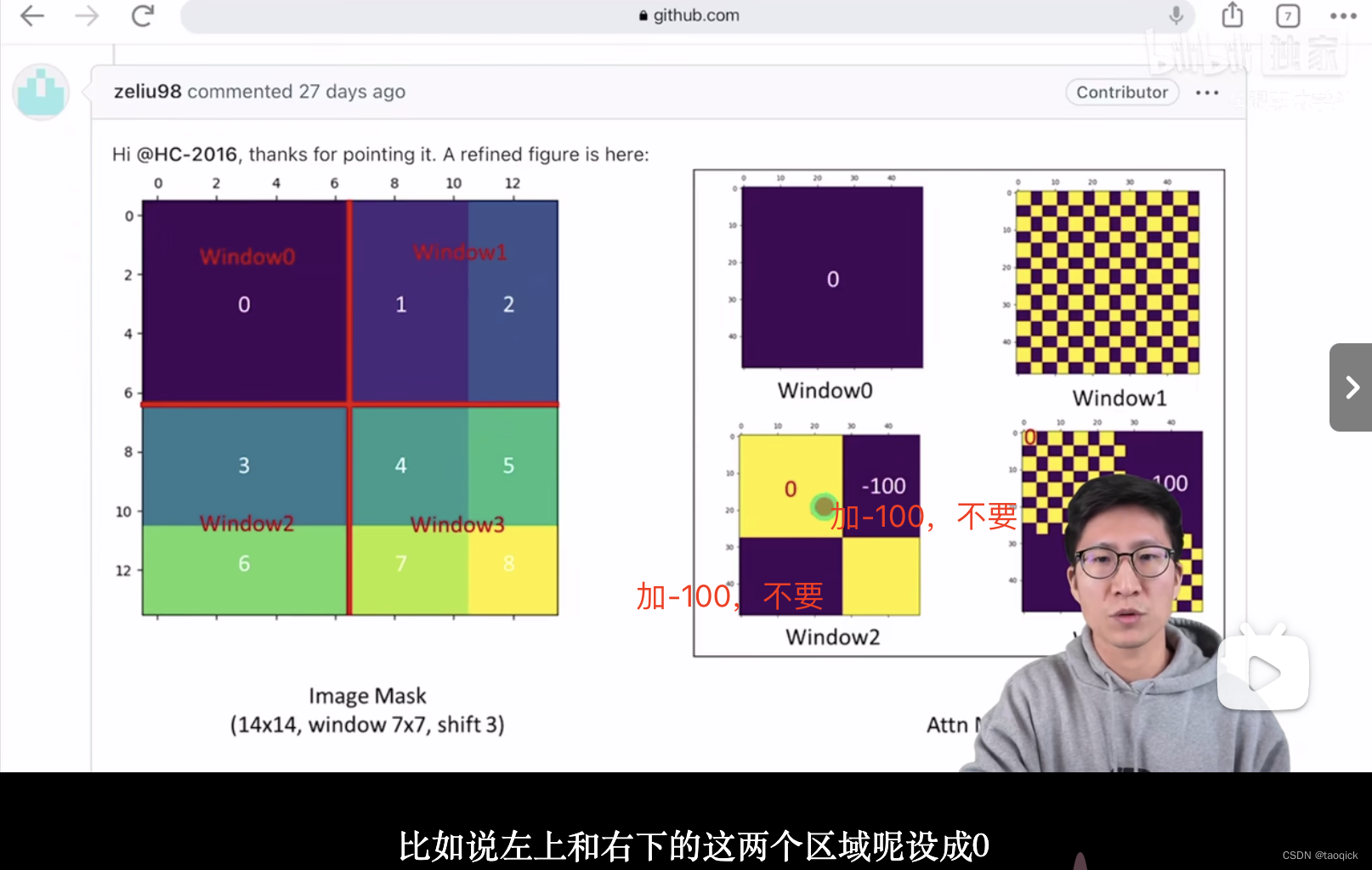
Attention Mask
我认为这是Swin Transformer的精华,通过设置合理的mask模版,让Shifted Window Attention在与Window Attention相同的窗口个数下,达到等价的计算结果。这部分Yi Zhu老师视频讲的比较清楚:
代码实现:
        if self.shift_size > 0:
            # calculate attention mask for SW-MSA
            H, W = self.input_resolution
            img_mask = torch.zeros((1, H, W, 1))  # 1 H W 1
            h_slices = (slice(0, -self.window_size),
                        slice(-self.window_size, -self.shift_size),
                        slice(-self.shift_size, None))
            w_slices = (slice(0, -self.window_size),
                        slice(-self.window_size, -self.shift_size),
                        slice(-self.shift_size, None))
            cnt = 0
            for h in h_slices:
                for w in w_slices:
                    img_mask[:, h, w, :] = cnt
                    cnt += 1

            mask_windows = window_partition(img_mask, self.window_size)  # nW, window_size, window_size, 1
            mask_windows = mask_windows.view(-1, self.window_size * self.window_size)
            attn_mask = mask_windows.unsqueeze(1) - mask_windows.unsqueeze(2)
            attn_mask = attn_mask.masked_fill(attn_mask != 0, float(-100.0)).masked_fill(attn_mask == 0, float(0.0))
'''
以上图的设置,我们用这段代码会得到这样的一个mask
tensor([[[[[   0.,    0.,    0.,    0.],
           [   0.,    0.,    0.,    0.],
           [   0.,    0.,    0.,    0.],
           [   0.,    0.,    0.,    0.]]],


         [[[   0., -100.,    0., -100.],
           [-100.,    0., -100.,    0.],
           [   0., -100.,    0., -100.],
           [-100.,    0., -100.,    0.]]],


         [[[   0.,    0., -100., -100.],
           [   0.,    0., -100., -100.],
           [-100., -100.,    0.,    0.],
           [-100., -100.,    0.,    0.]]],


         [[[   0., -100., -100., -100.],
           [-100.,    0., -100., -100.],
           [-100., -100.,    0., -100.],
           [-100., -100., -100.,    0.]]]]])
'''
在之前的window attention模块的前向代码里,包含这么一段
        if mask is not None:
            nW = mask.shape[0]
            attn = attn.view(B_ // nW, nW, self.num_heads, N, N) + mask.unsqueeze(1).unsqueeze(0)
            attn = attn.view(-1, self.num_heads, N, N)
            attn = self.softmax(attn)
将mask加到attention的计算结果,并进行softmax。mask的值设置为-100,softmax后就会忽略掉对应的值
SwinTransformerBlock
Swin-B: C = 128, layer numbers ={2; 2; 18; 2}
除去最后一层stage外,其他每个stage中都是先进行W-MSA,然后进行SW-MSA。
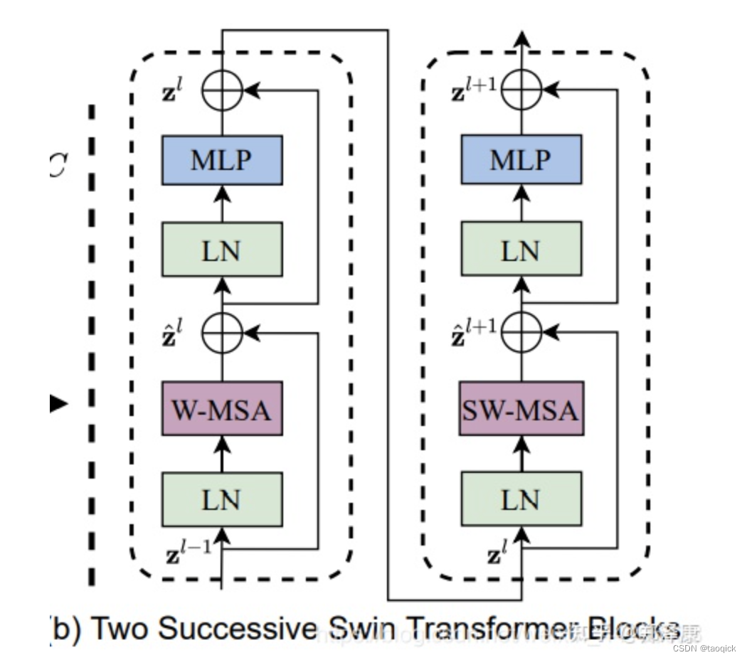
两个连续的Block架构如上图所示,需要注意的是一个Stage包含的Block个数必须是偶数,因为需要交替包含一个含有Window Attention的Layer和含有Shifted Window Attention的Layer。
我们看下Block的前向代码
    def forward(self, x):
        H, W = self.input_resolution
        B, L, C = x.shape
        assert L == H * W, "input feature has wrong size"

        shortcut = x
        x = self.norm1(x)
        x = x.view(B, H, W, C)

        # cyclic shift
        if self.shift_size > 0:
            shifted_x = torch.roll(x, shifts=(-self.shift_size, -self.shift_size), dims=(1, 2))
        else:
            shifted_x = x

        # partition windows
        x_windows = window_partition(shifted_x, self.window_size)  # nW*B, window_size, window_size, C
        x_windows = x_windows.view(-1, self.window_size * self.window_size, C)  # nW*B, window_size*window_size, C

        # W-MSA/SW-MSA
        attn_windows = self.attn(x_windows, mask=self.attn_mask)  # nW*B, window_size*window_size, C

        # merge windows
        attn_windows = attn_windows.view(-1, self.window_size, self.window_size, C)
        shifted_x = window_reverse(attn_windows, self.window_size, H, W)  # B H' W' C

        # reverse cyclic shift
        if self.shift_size > 0:
            x = torch.roll(shifted_x, shifts=(self.shift_size, self.shift_size), dims=(1, 2))
        else:
            x = shifted_x
        x = x.view(B, H * W, C)

        # FFN
        x = shortcut + self.drop_path(x)
        x = x + self.drop_path(self.mlp(self.norm2(x)))

        return x
本文感谢并进行了部分转载:
- SwinTransformer的paper:https://arxiv.org/pdf/2103.14030.pdf
- Vit的paper:https://arxiv.org/pdf/2010.11929.pdf
- https://zhuanlan.zhihu.com/p/367111046
- 【Swin Transformer论文精读【论文精读】】https://www.bilibili.com/video/BV13L4y1475U?vd_source=e260233b721e72ff23328d5f4188b304


 1536
1536


 被折叠的 条评论
为什么被折叠?
被折叠的 条评论
为什么被折叠?
 到【灌水乐园】发言


