曲线拟合

scipy的小应用  ：《机器学习系统设计》

对web_traffic数据拟合

# coding=utf-8
# 导入包
import os
import scipy as sp
import matplotlib.pyplot as plt

# 导入数据
data = sp.genfromtxt("web_traffic.tsv", delimiter="\t")
#print(data[: 10])

# all examples will have three classes in this file
colors = ['g', 'k', 'm', 'b', 'r']
linestyles = ['-', '-.', '--', ':', '-']

x = data[:, 0]
y = data[:, 1]

x = x[~sp.isnan(y)]
y = y[~sp.isnan(y)]

# 画出散点图

def plot_models(x, y, models, fname, mx=None, ymax=None, xmin=None):
    plt.clf()
    plt.scatter(x, y, s=10, color='y')
    plt.title("Web traffic over the last month")
    plt.xlabel("Time")
    plt.ylabel("Hits/hour")
    plt.xticks(
        [w * 7 * 24 for w in range(10)], ['week %i' % w for w in range(10)])

    if models:
        if mx is None:
            mx = sp.linspace(0, x[-1], 1000)
        for model, style, color in zip(models, linestyles, colors):
            # print "Model:",model
            # print "Coeffs:",model.coeffs
            plt.plot(mx, model(mx), linestyle=style, linewidth=2, c=color)

        plt.legend(["d=%i" % m.order for m in models], loc="upper left")

    plt.autoscale(tight=True)
    plt.ylim(ymin=0)
    if ymax:
        plt.ylim(ymax=ymax)
    if xmin:
        plt.xlim(xmin=xmin)
    plt.grid(True, linestyle='-', color='0.75')
    plt.savefig(fname)


# 定义误差函数
def error(f, x, y):
    return sp.sum((f(x)-y)**2)

#---------------------------------------------------------#

# 用一阶模型拟合
fp1, residuals, rank, sv, rcond = sp.polyfit(x, y, 1, full=True)
print("Model parameters: %s" % fp1)

# 根据这些参数创造模型函数
f1 = sp.poly1d(fp1)
print(error(f1, x, y))

# 画出训练后的模型
#fx = sp.linspace(0, x[-1], 1000)
#plt.plot(fx, f1(fx), linewidth=4)
#plt.legend(["d=%i" % f1.order], loc="upper left")

#----------------------------------------------------------#
# 用二阶模型拟合
f2p = sp.polyfit(x, y, 2)
print("Model parameters: %s" % f2p)

f2 = sp.poly1d(f2p)
print(error(f2, x, y))

#----------------------------------------------------------#
# 用三阶模型拟合
f3p = sp.polyfit(x, y, 3)
print("Model parameters: %s" % f3p)

f3 = sp.poly1d(f3p)
print(error(f3, x, y))

#----------------------------------------------------------#
# 用100阶模型拟合
fhp = sp.polyfit(x, y, 100)
print("Model parameters: %s" % fhp)

f100 = sp.poly1d(fhp)
print(error(f100, x, y))


# 画出图像并将图像保存在当前目录
plot_models(x, y, None, os.path.join("", "1_00.png"))
plot_models(x, y, [f1], os.path.join("", "1_01.png"))
plot_models(x, y, [f1, f2], os.path.join("", "1_02.png"))
plot_models(x, y, [f1, f2, f3], os.path.join("", "1_03.png"))
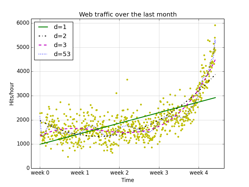
plot_models(x, y, [f1, f2, f3, f100], os.path.join("", "1_04.png"))

结果如图：