Tensorflow - Tutorial (4) :基于CNN的手写数字识别

1. 模型结构

本文只涉及利用Tensorflow实现CNN的手写数字识别,关于CNN的内容请参考:卷积神经网络(CNN)

MNIST数据集的格式与数据预处理代码input_data.py的讲解请参考 :Tutorial (2)

该CNN模型包含3个卷积层,2个全连接层,具体结构如下:

• 输入层 : CNN的输入是一张图片,用28x28的矩阵表示
• C1层 :该层为卷积层,卷积核大小是3x3,激活函数为RELU.输入一个28x28的矩阵,输出32个28x28 维的feature map
• S1层 :该层为max pooling层,窗口大小是2x2,输入32个28x28的矩阵,输出32个14x14 维的feature map
• C2层 :该层为卷积层,卷积核大小是3x3,激活函数为RELU.输入32个14x14的feature map,输出64个14x14 的feature map
• S2层 :该层为max pooling层,窗口大小是2x2,输入64个14x14 的feature map,输出64个7x7 的feature map
• C3层 :该层为卷积层,卷积核大小是3x3,激活函数为RELU.输入64个7x7 的feature map,输出128个7x7 的feature map
• S3层 :该层为max pooling层,窗口大小是2x2,输入128个7x7 的feature map,输出128个4x4 的feature map,并将这128个feature map合并为一个128x4x4=2048维的向量
• F4层 :该层为全连接层,神经元个数为625
• F5层 :该层为全连接层,输出一个10维向量,表示label的概率分布

2. 实验代码

实验代码如下:

#!/usr/bin/env python

import tensorflow as tf
import numpy as np
import input_data

batch_size = 128
test_size = 256
#初始化参数
def init_weights(shape):
    return tf.Variable(tf.random_normal(shape, stddev=0.01))
'''
tensorflow中conv2d的"padding"参数可以设为两个值SAME，VALID
它们对边界是这样处理的，对输入的矩阵，包裹n层0，然后再按照上面所说的卷积方法进行卷积，n的求法:

SAME: edge_row = (kernel_row - 1) / 2;   edge_cols = (kernel_cols - 1) / 2; 
VALID:edge_row = edge_cols = 0;  

edge_row就是包裹0的行数，edge_cols就是包裹0的列数, kernel_row就是卷积核的行数
'''
def model(X, w, w2, w3, w4, w_o, p_keep_conv, p_keep_hidden):
    #第一个卷积层:padding=SAME,保证输出的feature map与输入矩阵的大小相同
    l1a = tf.nn.relu(tf.nn.conv2d(X, w,                       # l1a shape=(?, 28, 28, 32)
                        strides=[1, 1, 1, 1], padding='SAME'))
    #max_pooling,窗口大小为2x2
    l1 = tf.nn.max_pool(l1a, ksize=[1, 2, 2, 1],              # l1 shape=(?, 14, 14, 32)
                        strides=[1, 2, 2, 1], padding='SAME')
    #dropout:每个神经元有p_keep_conv的概率以1/p_keep_conv的比例进行归一化,有(1-p_keep_conv)的概率置为0
    l1 = tf.nn.dropout(l1, p_keep_conv)

    #第二个卷积层
    l2a = tf.nn.relu(tf.nn.conv2d(l1, w2,                     # l2a shape=(?, 14, 14, 64)
                        strides=[1, 1, 1, 1], padding='SAME'))
    l2 = tf.nn.max_pool(l2a, ksize=[1, 2, 2, 1],              # l2 shape=(?, 7, 7, 64)
                        strides=[1, 2, 2, 1], padding='SAME')
    l2 = tf.nn.dropout(l2, p_keep_conv)

    #第三个卷积层
    l3a = tf.nn.relu(tf.nn.conv2d(l2, w3,                     # l3a shape=(?, 7, 7, 128)
                        strides=[1, 1, 1, 1], padding='SAME'))
    l3 = tf.nn.max_pool(l3a, ksize=[1, 2, 2, 1],              # l3 shape=(?, 4, 4, 128)
                        strides=[1, 2, 2, 1], padding='SAME')
    #将所有的feature map合并成一个2048维向量
    l3 = tf.reshape(l3, [-1, w4.get_shape().as_list()[0]])    # reshape to (?, 2048)
    l3 = tf.nn.dropout(l3, p_keep_conv)
    #后面两层为全连接层
    l4 = tf.nn.relu(tf.matmul(l3, w4))
    l4 = tf.nn.dropout(l4, p_keep_hidden)

    pyx = tf.matmul(l4, w_o)
    return pyx

mnist = input_data.read_data_sets("MNIST_data/", one_hot=True)#读取数据
#mnist.train.images是一个55000 * 784维的矩阵, mnist.train.labels是一个55000 * 10维的矩阵
trX, trY, teX, teY = mnist.train.images, mnist.train.labels, mnist.test.images, mnist.test.labels
trX = trX.reshape(-1, 28, 28, 1)  # 将每张图片用一个28x28的矩阵表示,(55000,28,28,1)
teX = teX.reshape(-1, 28, 28, 1)  # 将每张图片用一个28x28的矩阵表示,(1000,28,28,1)

X = tf.placeholder("float", [None, 28, 28, 1])
Y = tf.placeholder("float", [None, 10])

w = init_weights([3, 3, 1, 32])       # 第一层卷积核大小为3x3,输入一张图,输出32个feature map
w2 = init_weights([3, 3, 32, 64])     # 第二层卷积核大小为3x3,输入32个feature map,输出64个feature map
w3 = init_weights([3, 3, 64, 128])    # 第三层卷积核大小为3x3,输入64个feature map,输出128个feature map
w4 = init_weights([128 * 4 * 4, 625]) # FC 128 * 4 * 4 inputs, 625 outputs
w_o = init_weights([625, 10])         # FC 625 inputs, 10 outputs (labels)

p_keep_conv = tf.placeholder("float") # 卷积层的dropout概率
p_keep_hidden = tf.placeholder("float")# 全连接层的dropout概率
py_x = model(X, w, w2, w3, w4, w_o, p_keep_conv, p_keep_hidden)

cost = tf.reduce_mean(tf.nn.softmax_cross_entropy_with_logits(py_x, Y))# 交叉熵目标函数
train_op = tf.train.RMSPropOptimizer(0.001, 0.9).minimize(cost)#RMSPro算法最小化目标函数
predict_op = tf.argmax(py_x, 1)#返回每个样本的预测结果

# Launch the graph in a session
with tf.Session() as sess:
    # you need to initialize all variables
    tf.initialize_all_variables().run()

    for i in range(100):
        training_batch = zip(range(0, len(trX), batch_size),
                             range(batch_size, len(trX)+1, batch_size))
        for start, end in training_batch:
            sess.run(train_op, feed_dict={X: trX[start:end], Y: trY[start:end],
                                          p_keep_conv: 0.8, p_keep_hidden: 0.5})
        #test
        test_indices = np.arange(len(teX)) 
        np.random.shuffle(test_indices)
        test_indices = test_indices[0:test_size]#选取一批测试数据

        print(i, np.mean(np.argmax(teY[test_indices], axis=1) ==
                         sess.run(predict_op, feed_dict={X: teX[test_indices],
                                                         Y: teY[test_indices],
                                                         p_keep_conv: 1.0,
                                                         p_keep_hidden: 1.0})))

3. 结果

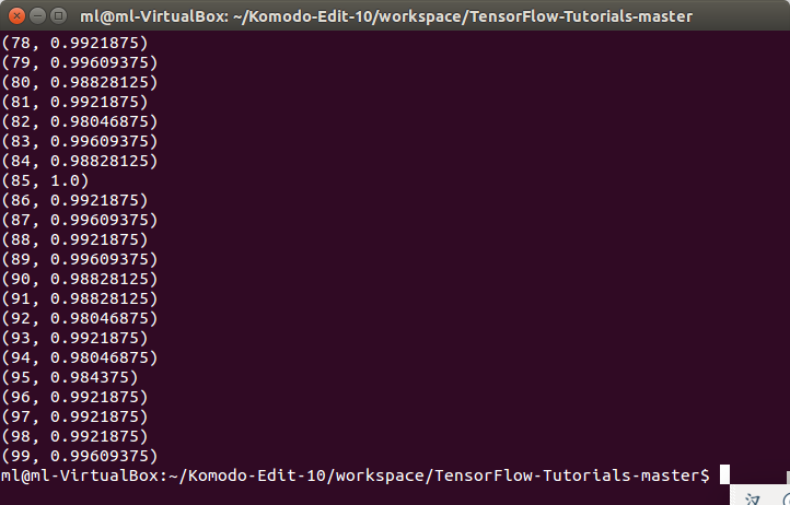
基于CNN的手写数字识别准确率可达到99.6%,与softmax模型(91%)和普通的NN(95%)模型相比,性能有了较大提升.