循环神经网络RNN 2—— attention注意力机制（附代码）

最新推荐文章于 2025-04-01 12:53:37 发布

端坐的小王子

最新推荐文章于 2025-04-01 12:53:37 发布

阅读量7.4k

点赞数 11

分类专栏： NLP 推荐系统文章标签： rnn 深度学习 nlp

本文链接：https://blog.csdn.net/u012290039/article/details/106768381

版权

推荐系统同时被 2 个专栏收录

21 篇文章

订阅专栏

NLP

6 篇文章

订阅专栏

attention方法是一种注意力机制，很明显，是为了模仿人的观察和思维方式，将注意力集中到关键信息上，虽然还没有像人一样，完全忽略到不重要的信息，但是其效果毋庸置疑，本篇我们来总结注意力机制的不同方法。
循环神经网络RNN 1—— 基本模型及其变体
 循环神经网络RNN 2—— attention注意力机制（附代码）
循环神经网络RNN 3——LSTM及其变体

1，attention的定义

我们先给出定义，后面给出attention的多种实现方法，带着问题来学习和实践。

1）给定一组向量集合values，以及一个向量query，那么attention机制就是一种根据该query计算values的加权求和的机制。这里query看做是decode的h，values看做是encode的h。
2）attention的重点就是这个集合values中的每个value的“权值”的计算方法。
3）有时候也把这种attention的机制叫做query的输出关注了（或者说叫考虑到了）原文的不同部分（Query attends to the values），因为这其中有对encode加权部分。

2，基础的attention

在Encoder-Decoder结构中，Encoder把所有的输入序列都编码成一个统一的语义特征c再解码，因此， c中必须包含原始序列中的所有信息，它的长度就成了限制模型性能的瓶颈。如机器翻译问题，当要翻译的句子较长时，一个c可能存不下那么多信息，就会造成翻译精度的下降。

Attention机制通过在每个时间输入不同的c来解决这个问题，下图是带有Attention机制的Decoder（注意，是解码部分）：
在这里插入图片描述
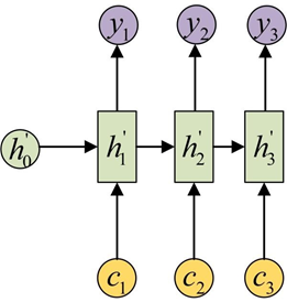
每一个c会自动去选取与当前所要输出的y最合适的上下文信息。具体来说，我们用 $a_{ij}$ 衡量Encoder中第j阶段的 $h_j$ 和解码时第i阶段的相关性，最终Decoder中第i阶段的输入的上下文信息 $c_i$ 就来自于所有hi对 $a_{ij}$ 的加权和。
以机器翻译为例（将中文翻译成英文）：
在这里插入图片描述
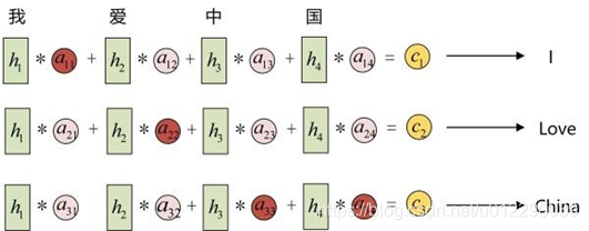
输入的序列是“我爱中国”，因此，Encoder中的h1、h2、h3、h4就可以分别看做是“我”、“爱”、“中”、“国”所代表的信息。在翻译成英语时，第一个上下文c1应该和“我”这个字最相关，因此对应的 a11 就比较大，而相应的 a12、a13、a14 就比较小。c2应该和“爱”最相关，因此对应的 a22 就比较大。最后的c3和h3、h4最相关，因此 a33 、 a34的值就比较大。

至此，关于Attention模型，我们就只剩最后一个问题了，那就是：这些权重 $a_{ij}$ 是怎么来的？

事实上， $a_{ij}$ 同样是从模型中学出的，它实际和Decoder的第i-1阶段的隐状态、Encoder第j个阶段的隐状态有关。

同样还是拿上面的机器翻译举例， $a_{1j}$ 、 $a_{1j}$ 的计算（此时箭头就表示对h’和 hj 同时做变换）：
在这里插入图片描述
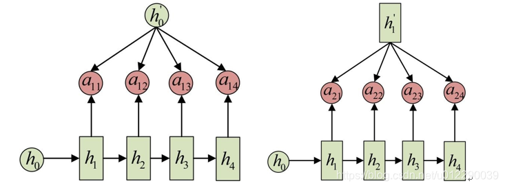
这个过程如何计算呢？ 其实思路很简单：

我们在encoder的过程中保留每个RNN单元的隐藏状态（hidden state）得到 $h_1……h_N）$
此时假设decode的time-step为t，那么将decode前一个隐藏状态 $h_{t-1}'$ ,与 $h_1……h_N$ 相乘，得到attention score，成为相似度或者“影响度”，或者“匹配得分”.
在这里插入图片描述
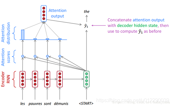
然后利用softmax，将attention scores转化为概率分布，按照刚才的概率分布，计算encoder的hidden states的加权求和。
$a_t = \sum_i^N\alpha_ih_i$
attention计算完成， $a_t$ 就是decoder的第t时刻的注意力向量。然后将 $a_t$ 与decode时刻的hidden state并联起来，做后续处理，比如分类等。

3, attention变体

根据以上分析，attention主要分为两部分，score值的计算，权值的计算，剩下的就是加权，所以attention的变体也是围绕着这两个方面来的。一种是在attention 向量的加权求和计算方式上进行创新；一种是在attention score（匹配度或者叫权值）的计算方式上进行创新。

3.1，针对attention向量计算方式的变体

3.1.1 Soft-attention

在这里插入图片描述
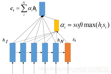
这是一种基本的attention结构，先通过点乘获得attention score，经过softmax得到alpha权值，然后加权求和得到attention变量（context vecor）
论文：Neural machine translation by jointly learning to align and translate

3.1.2 Hard attention

在这里插入图片描述
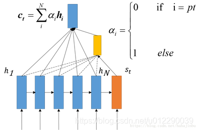
区别于soft attention，hard-attention寻找特定的h与之相应的timestep对齐。

3.1.3 Local attention

在这里插入图片描述

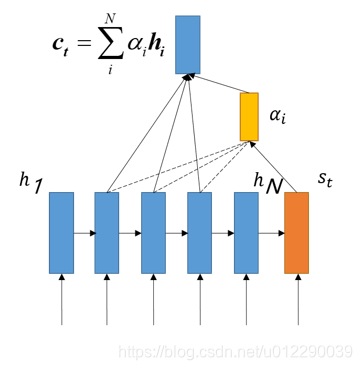
Local-attention介于soft-attention与hard-attention之间，取一个窗口，对窗口内的数据进行加权。

方式有两种：
一种是线性对齐，假设对齐位置pt=t，然后计算窗口内的softmax。
$\alpha_i=\frac{exp(score(h'_i,s_i))}{\sum_i exp(score(h'_i,s_i))}$
另一种是通过一个函数预测pt的位置.
$\begin{aligned} & p_t=S*sigmoid(V_p^t*tanh(W_p*s_t)) \\ & \alpha_t = \frac{exp(score(h'_i,s_i))}{\sum_i exp(score(h'_i,s_i))}*exp(-frac{(s-p_t)}{2\sigma^2}) \end{aligned}$
S表示源句子长度大小， $W_p$ 与 $V_p$ 表示模型参数通过训练得到，为了得到 $p_t$ 附近的对齐点，设置一个围绕 $p_t$ 的高斯分布，s是在以 $p_t$ 为中心的窗口中的整数。 $p_t$ 是一个在[0，S]之间的实数. σ 一般取窗口大小的一半.

3.2, 针对attention score计算方式的变体

在计算权值向量之前，我们要计算出attention score.
$\begin{aligned} & \alpha = softmax(e)\\ & a = \sum_{i=1}^{N}\alpha_ih_i \end{aligned}$
attention score的计算方式有多种:
点积：
$e_i = s^T*h_i$
这里有个假设，就是s和h的维数要一样才能进行点积
乘法
$e_i = s^T*W*h_i$
W矩阵是训练得到的参数，维度是d2 x d1，d2是s的hidden state输出维数，d1是hi的hidden state维数。
加法
$e_i = v^T*tanh(W_1h_i+W_2s)$
additive attention，是对两种hidden state 分别再训练矩阵然后激活过后再乘以一个参数向量变成一个得分。其中，W1 = d3xd1，W2 = d3*d2，v = d3x1 ，d1，d2，d3分别为h和s还有v的维数，属于超参数。

3.3 self-attention

Self attention也叫做intra-attention在没有任何额外信息的情况下，我们仍然可以通过允许句子使用–self attention机制来处理自己，从句子中提取关注信息。

方法一：以当前的隐藏状态去计算和前面的隐藏状态的得分，作为当前隐藏单元的attention score:
$e_{h_i}=h_t^T*W*h_i$

方法二：以当前状态本身去计算得分作为当前单元attention score，这种方式更常见，也更简单，例如：

$\begin{aligned} & e_{h_i}=v_{\alpha}^{T}tanh(w_{\alpha}h_i)\\ & e_{h_i} = tanh(w^Th_i+b) \end{aligned}$

#coding=utf-8
'''
Single model may achieve LB scores at around 0.043
Don't need to be an expert of feature engineering
All you need is a GPU!!!!!!!

The code is tested on Keras 2.0.0 using Theano backend, and Python 3.5

referrence Code:https://www.kaggle.com/lystdo/lstm-with-word2vec-embeddings
'''

########################################
## import packages
########################################
import os
import re
import csv
import codecs
import numpy as np
import pandas as pd

########################################
## set directories and parameters
########################################



from keras import backend as K
from keras.engine.topology import Layer
# from keras import initializations
from keras import initializers, regularizers, constraints

np.random.seed(2018)

class Attention(Layer):
    def __init__(self,
                 W_regularizer=None, b_regularizer=None,
                 W_constraint=None, b_constraint=None,
                 bias=True, **kwargs):
        """
        Keras Layer that implements an Attention mechanism for temporal data.
        Supports Masking.
        Follows the work of Raffel et al. [https://arxiv.org/abs/1512.08756]
        # Input shape
            3D tensor with shape: `(samples, steps, features)`.
        # Output shape
            2D tensor with shape: `(samples, features)`.
        :param kwargs:

        """
        self.supports_masking = True
        # self.init = initializations.get('glorot_uniform')
        self.init = initializers.get('glorot_uniform')

        self.W_regularizer = regularizers.get(W_regularizer)
        self.b_regularizer = regularizers.get(b_regularizer)

        self.W_constraint = constraints.get(W_constraint)
        self.b_constraint = constraints.get(b_constraint)

        self.bias = bias

        self.features_dim = 0
        super(Attention, self).__init__(**kwargs)

    def build(self, input_shape):
        self.step_dim = input_shape[1]
        assert len(input_shape) == 3 # batch ,timestep , num_features
        print(input_shape)
        self.W = self.add_weight((input_shape[-1],), #num_features
                                 initializer=self.init,
                                 name='{}_W'.format(self.name),
                                 regularizer=self.W_regularizer,
                                 constraint=self.W_constraint)
        self.features_dim = input_shape[-1]

        if self.bias:
            self.b = self.add_weight((input_shape[1],),#timesteps
                                     initializer='zero',
                                     name='{}_b'.format(self.name),
                                     regularizer=self.b_regularizer,
                                     constraint=self.b_constraint)
        else:
            self.b = None

        self.built = True

    def compute_mask(self, input, input_mask=None):
        # do not pass the mask to the next layers
        return None

    def call(self, x, mask=None):
        features_dim = self.features_dim
        step_dim = self.step_dim
        print(K.reshape(x, (-1, features_dim)))# n, d
        print(K.reshape(self.W, (features_dim, 1)))# w= dx1
        print(K.dot(K.reshape(x, (-1, features_dim)), K.reshape(self.W, (features_dim, 1))))#nx1

        eij = K.reshape(K.dot(K.reshape(x, (-1, features_dim)), K.reshape(self.W, (features_dim, 1))), (-1, step_dim))#batch,step
        print(eij)
        if self.bias:
            eij += self.b

        eij = K.tanh(eij)

        a = K.exp(eij)

        # apply mask after the exp. will be re-normalized next
        if mask is not None:
            # Cast the mask to floatX to avoid float64 upcasting in theano
            a *= K.cast(mask, K.floatx())

        a /= K.cast(K.sum(a, axis=1, keepdims=True) + K.epsilon(), K.floatx())
        print(a)
        a = K.expand_dims(a)
        print("expand_dims:")
        print(a)
        print("x:")
        print(x)
        weighted_input = x * a
        print(weighted_input.shape)
        return K.sum(weighted_input, axis=1)

    def compute_output_shape(self, input_shape):
        # return input_shape[0], input_shape[-1]
        return input_shape[0], self.features_dim

3.3 multi-head attention

在这里插入图片描述
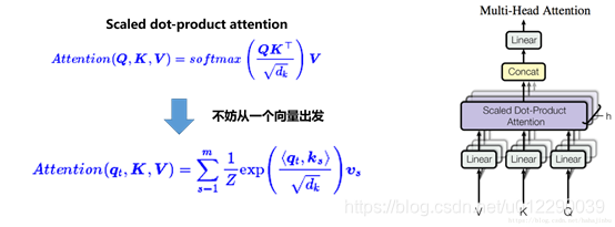
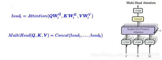
Google 在 attention is all you need 中发明了一种叫transformer的网络结构，其中用到了multi-head attention。

首先，google先定义了一下attention的参数 key，value，query三个元素（在seq2seq里面，query是st，key和value都是hi）在self 里面，query 是当前要计算的hi，k和v仍然一样，是其他单元的hidden state。在key value attention里面key和value则是分开了的。）

整个过程仍然没有脱离attention的基本结构，计算attention_score，然后得到权值，加权求和，不过这里可以设置多个head1组合在一起。

class MultiHeadAttention(Layer):

    def __init__(self, n_heads, head_dim, dropout_rate=.1, masking=True, future=False, trainable=True, **kwargs):
        self._n_heads = n_heads
        self._head_dim = head_dim
        self._dropout_rate = dropout_rate
        self._masking = masking
        self._future = future
        self._trainable = trainable
        super(MultiHeadAttention, self).__init__(**kwargs)

    def build(self, input_shape):
        self._weights_queries = self.add_weight(
            shape=(input_shape[0][-1], self._n_heads * self._head_dim),
            initializer='glorot_uniform',
            trainable=self._trainable,
            name='weights_queries')
        self._weights_keys = self.add_weight(
            shape=(input_shape[1][-1], self._n_heads * self._head_dim),
            initializer='glorot_uniform',
            trainable=self._trainable,
            name='weights_keys')
        self._weights_values = self.add_weight(
            shape=(input_shape[2][-1], self._n_heads * self._head_dim),
            initializer='glorot_uniform',
            trainable=self._trainable,
            name='weights_values')
        super(MultiHeadAttention, self).build(input_shape)


    def call(self, inputs):
        if self._masking:
            assert len(inputs) == 4, "inputs should be set [queries, keys, values, masks]."
            queries, keys, values, masks = inputs
        else:
            assert len(inputs) == 3, "inputs should be set [queries, keys, values]."
            queries, keys, values = inputs
        
        queries_linear = K.dot(queries, self._weights_queries) 
        keys_linear = K.dot(keys, self._weights_keys)
        values_linear = K.dot(values, self._weights_values)

        queries_multi_heads = tf.concat(tf.split(queries_linear, self._n_heads, axis=2), axis=0)
        keys_multi_heads = tf.concat(tf.split(keys_linear, self._n_heads, axis=2), axis=0)
        values_multi_heads = tf.concat(tf.split(values_linear, self._n_heads, axis=2), axis=0)
        
        if self._masking:
            att_inputs = [queries_multi_heads, keys_multi_heads, values_multi_heads, masks]
        else:
            att_inputs = [queries_multi_heads, keys_multi_heads, values_multi_heads]
            
        attention = ScaledDotProductAttention(
            masking=self._masking, future=self._future, dropout_rate=self._dropout_rate)
        att_out = attention(att_inputs)

        outputs = tf.concat(tf.split(att_out, self._n_heads, axis=0), axis=2)
        
        return outputs

    def compute_output_shape(self, input_shape):
        return input_shape

4，总结
综合来看，attention的机制就是一个加权求和的机制，不管是什么变体目前都没有离开这个思路，只要根据已有信息计算的隐藏状态的加权和求和，那么就是使用了attention。self attention就是仅仅在句子内部做加权求和（区别与seq2seq里面的decoder对encoder的隐藏状态做的加权求和），key-value attention是将h分开，很多模型中都可以借鉴key-value方法，比如可以将key-value看作是一样的，multi-attention看成多核并联就好了。

参考资料：

https://www.leiphone.com/news/201709/8tDpwklrKubaecTa.html
https://blog.csdn.net/hahajinbu/article/details/81940355
https://zhuanlan.zhihu.com/p/67115572
https://zhuanlan.zhihu.com/p/118503318
https://zhuanlan.zhihu.com/p/116091338
https://blog.csdn.net/xiaosongshine/article/details/86595847