Stochastic Optimization Techniques随机优化相关笔记

• skip to content

http://colinraffel.com/wiki/

User Tools

• Log In

Site Tools

• Recent Changes
• Media Manager
• Sitemap

---

stochastic_optimization_techniques

Table of Contents

Paper summaries,Neural Networks,Optimization

Stochastic Optimization Techniques

Neural networks are often trained stochastically, i.e. using a method where the objective function changes at each iteration. This stochastic variation is due to the model being trained on different data during each iteration. This is motivated by (at least) two factors: First, the dataset used as training data is often too large to fit in memory and/or be optimized over efficiently. Second, the objective function is typically nonconvex, so using different data at each iteration can help prevent the model from settling in a local minimum. Furthermore, training neural networks is usually done using only the first-order gradient of the parameters with respect to the loss function. This is due to the large number of parameters present in a neural network, which for practical purposes prevents the computation of the Hessian matrix. Because vanilla gradient descent can diverge or converge incredibly slowly if its learning rate hyperparameter is set inappropriately, many alternative methods have been proposed which are intended to produce desirable convergence with less dependence on hyperparameter settings. These methods often effectively compute and utilize a preconditioner on the gradient, adaptively change the learning rate over time or approximate the Hessian matrix.

In the following, we will use θt to denote some generic parameter of the model at iteration t , to be optimized according to some loss function L which is to be minimized.

Stochastic Gradient Descent

Stochastic gradient descent (SGD) simply updates each parameter by subtracting the gradient of the loss with respect to the parameter, scaled by the learning rate η , a hyperparameter. If η is too large, SGD will diverge; if it's too small, it will converge slowly. The update rule is simply

θt+1=θt−η∇L(θt)

Momentum

In SGD, the gradient ∇L(θt) often changes rapidly at each iteration t due to the fact that the loss is being computed over different data. This is often partially mitigated by re-using the gradient value from the previous iteration, scaled by a momentum hyperparameter μ , as follows:

vt+1θt+1=μvt−η∇L(θt)=θt+vt+1

It has been argued that including the previous gradient step has the effect of approximating some second-order information about the gradient.

Nesterov's Accelerated Gradient

In Nesterov's Accelerated Gradient (NAG), the gradient of the loss at each step is computed at θt+μvt instead of θt . In momentum, the parameter update could be written θt+1=θt+μvt−η∇L(θt) , so NAG effectively computes the gradient at the new parameter location but without considering the gradient term. In practice, this causes NAG to behave more stably than regular momentum in many situations. A more thorough analysis can be found in ¹⁾. The update rules are then as follows:

vt+1θt+1=μvt−η∇L(θt+μvt)=θt+vt+1

，牛顿法是二阶收敛，梯度下降是一阶收敛，所以牛顿法就更快。如果更通俗地说的话，比如你想找一条最短的路径走到一个盆地的最底部，梯度下降法每次只从你当前所处位置选一个坡度最大的方向走一步，牛顿法在选择方向时，不仅会考虑坡度是否够大，还会考虑你走了一步之后，坡度是否会变得更大。所以，可以说牛顿法比梯度下降法看得更远一点，能更快地走到最底部。

根据wiki上的解释，从几何上说，牛顿法就是用一个二次曲面去拟合你当前所处位置的局部曲面，而梯度下降法是用一个平面去拟合当前的局部曲面，通常情况下，二次曲面的拟合会比平面更好，所以牛顿法选择的下降路径会更符合真实的最优下降路径。

wiki上给的图很形象，我就直接转过来了： 红色的牛顿法的迭代路径，绿色的是梯度下降法的迭代路径。 红色的牛顿法的迭代路径，绿色的是梯度下降法的迭代路径。

参考：

http://en.wikipedia.org/wiki/Newton's_method_in_optimization

Adagrad

Adagrad effectively rescales the learning rate for each parameter according to the history of the gradients for that parameter. This is done by dividing each term in ∇L by the square root of the sum of squares of its historical gradient. Rescaling in this way effectively lowers the learning rate for parameters which consistently have large gradient values. It also effectively decreases the learning rate over time, because the sum of squares will continue to grow with the iteration. After setting the rescaling term g=0 , the updates are as follows:

gt+1θt+1=gt+∇L(θt)2=θt−η∇L(θt)gt+1−−−√+ϵ

where division is elementwise and ϵ is a small constant included for numerical stability. It has nice theoretical guarantees and empirical results ^{2) 3)}.

RMSProp

In its originally proposed form ⁴⁾, RMSProp is very similar to Adagrad. The only difference is that the gt term is computed as a exponentially decaying average instead of an accumulated sum. This makes gt an estimate of the second moment of ∇L and avoids the fact that the learning rate effectively shrinks over time. The name “RMSProp” comes from the fact that the update step is normalized by a decaying RMS of recent gradients. The update is as follows:

gt+1θt+1=γgt+(1−γ)∇L(θt)2=θt−η∇L(θt)gt+1−−−√+ϵ

In the original lecture slides where it was proposed, γ is set to .9 . In ⁵⁾, it is shown that the gt+1−−−√ term approximates (in expectation) the diagonal of the absolute value of the Hessian matrix (assuming the update steps are N(0,1) distributed). It is also argued that the absolute value of the Hessian is better to use for non-convex problems which may have many saddle points.

Alternatively, in ⁶⁾, a first-order moment approximator mt is added. It is included in the denominator of the preconditioner so that the learning rate is effectively normalized by the standard deviation ∇L . There is also a vt term included for momentum. This gives

mt+1gt+1vt+1θt+1=γmt+(1−γ)∇L(θt)=γgt+(1−γ)∇L(θt)2=μvt−η∇L(θt)gt+1−m2t+1+ϵ−−−−−−−−−−−−√=θt+vt+1

Adadelta

Adadelta ⁷⁾ uses the same exponentially decaying moving average estimate of the gradient second moment gt as RMSProp. It also computes a moving average xt of the updates vt similar to momentum, but when updating this quantity it squares the current step, which I don't have any intuition for.

gt+1vt+1xt+1θt+1=γgt+(1−γ)∇L(θt)2=−xt+ϵ−−−−−√∇L(θt)gt+1+ϵ−−−−−−√=γxt+(1−γ)v2t+1=θt+vt+1

Adam

Adam is somewhat similar to Adagrad/Adadelta/RMSProp in that it computes a decayed moving average of the gradient and squared gradient (first and second moment estimates) at each time step. It differs mainly in two ways: First, the first order moment moving average coefficient is decayed over time. Second, because the first and second order moment estimates are initialized to zero, some bias-correction is used to counteract the resulting bias towards zero. The use of the first and second order moments, in most cases, ensure that typically the gradient descent step size is ≈±η and that in magnitude it is less than η . However, as θt approaches a true minimum, the uncertainty of the gradient will increase and the step size will decrease. It is also invariant to the scale of the gradients. Given hyperparameters γ1 , γ2 , λ , and η , and setting m0=0 and g0=0 (note that the paper denotes γ1 as β1 , γ2 as β2 , η as α and gt as vt ), the update rule is as follows: ⁸⁾

mt+1gt+1m^t+1g^t+1θt+1=γ1mt+(1−γ1)∇L(θt)=γ2gt+(1−γ2)∇L(θt)2=mt+11−γt+11=gt+11−γt+12=θt−ηm^t+1g^t+1−−−−√+ϵ

ESGD

⁹⁾

Adasecant

¹⁰⁾

vSGD

¹¹⁾

Rprop

¹²⁾

¹⁾ Sutskever, Martens, Dahl, and Hinton, “On the importance of initialization and momentum in deep learning” (ICML 2013)

²⁾ Dyer, “Notes on AdaGrad”

³⁾ Duchi, Hazan, and Singer, “Adaptive Subgradient Methods for Online Learning and Stochastic Optimization” (COLT 2010)

⁴⁾ Hinton, Srivastava, and Swersky, “rmsprop: Divide the gradient by a running average of its recent magnitude”

⁵⁾ , ⁹⁾ Dauphin, Vries, Chung and Bengion, “RMSProp and equilibrated adaptive learning rates for non-convex optimization”

⁶⁾ Graves, “Generating Sequences with Recurrent Neural Networks”

⁷⁾ Zeiler, “Adadelta: An Adaptive Learning Rate Method”

⁸⁾ Kingma and Ba, “Adam: A Method for Stochastic Optimization”

¹⁰⁾ Gulcehre and Bengio, “Adasecant: Robust Adaptive Secant Method for Stochastic Gradient”

¹¹⁾ Schaul, Zhang, LeCun, “No More Pesky Learning Rates”

¹²⁾ Riedmiller and Bruan, “A Direct Adaptive Method for Faster Backpropagation Learning: The RPROP Algorithm”

]各种优化方法总结比较（sgd/momentum/Nesterov/adagrad/adadelta）

2015-12-5阅读1597 评论2

前言

这里讨论的优化问题指的是，给定目标函数f(x)，我们需要找到一组参数x，使得f(x)的值最小。

本文以下内容假设读者已经了解机器学习基本知识，和梯度下降的原理。

SGD

SGD指stochastic gradient descent，即随机梯度下降。是梯度下降的batch版本。

对于训练数据集，我们首先将其分成n个batch，每个batch包含m个样本。我们每次更新都利用一个batch的数据，而非整个训练集。即：

xt+1=xt+Δxt

Δxt=−ηgt

其中， η 为学习率， gt 为x在t时刻的梯度。

这么做的好处在于：

• 当训练数据太多时，利用整个数据集更新往往时间上不显示。batch的方法可以减少机器的压力，并且可以更快地收敛。
• 当训练集有很多冗余时（类似的样本出现多次），batch方法收敛更快。以一个极端情况为例，若训练集前一半和后一半梯度相同。那么如果前一半作为一个batch，后一半作为另一个batch，那么在一次遍历训练集时，batch的方法向最优解前进两个step，而整体的方法只前进一个step。

Momentum

SGD方法的一个缺点是，其更新方向完全依赖于当前的batch，因而其更新十分不稳定。解决这一问题的一个简单的做法便是引入momentum。

momentum即动量，它模拟的是物体运动时的惯性，即更新的时候在一定程度上保留之前更新的方向，同时利用当前batch的梯度微调最终的更新方向。这样一来，可以在一定程度上增加稳定性，从而学习地更快，并且还有一定摆脱局部最优的能力：

Δxt=ρxt−1−ηgt

其中， ρ 即momentum，表示要在多大程度上保留原来的更新方向，这个值在0-1之间，在训练开始时，由于梯度可能会很大，所以初始值一般选为0.5；当梯度不那么大时，改为0.9。 η 是学习率，即当前batch的梯度多大程度上影响最终更新方向，跟普通的SGD含义相同。 ρ 与 η 之和不一定为1。

Nesterov Momentum

这是对传统momentum方法的一项改进，由Ilya Sutskever(2012 unpublished)在Nesterov工作的启发下提出的。

其基本思路如下图（转自Hinton的coursera公开课lecture 6a）：

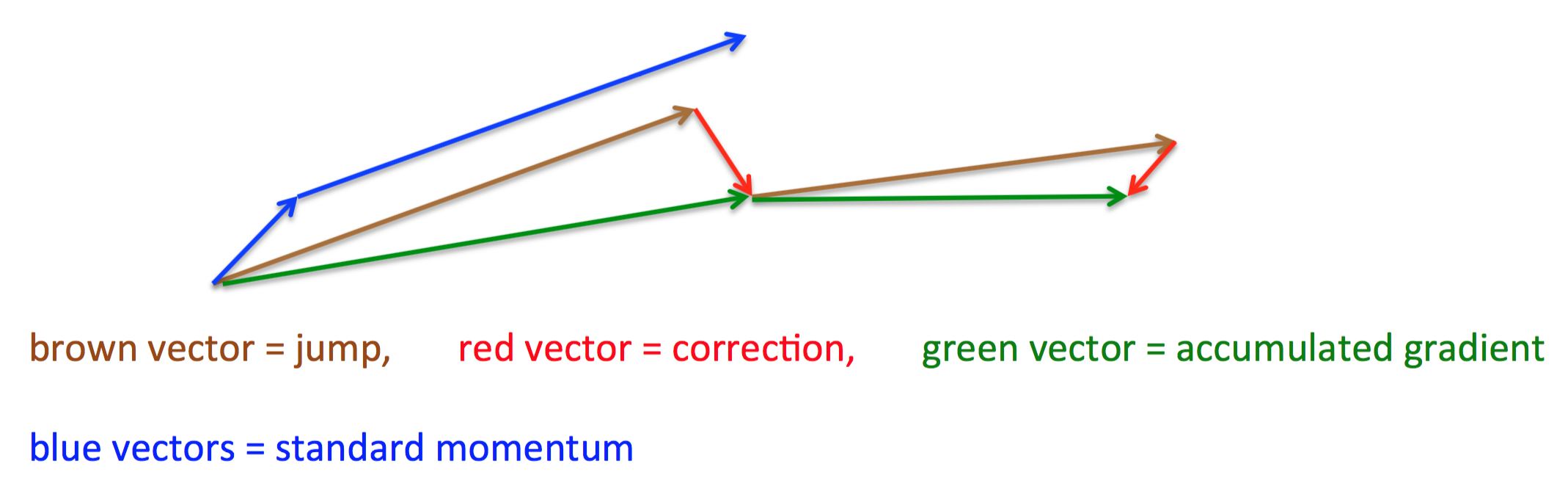
首先，按照原来的更新方向更新一步（棕色线），然后在该位置计算梯度值（红色线），然后用这个梯度值修正最终的更新方向（绿色线）。上图中描述了两步的更新示意图，其中蓝色线是标准momentum更新路径。

公式描述为：

Δxt=ρxt−1−ηΔf(xt−1+ρxt−1)

Adagrad

上面提到的方法对于所有参数都使用了同一个更新速率。但是同一个更新速率不一定适合所有参数。比如有的参数可能已经到了仅需要微调的阶段，但又有些参数由于对应样本少等原因，还需要较大幅度的调动。

Adagrad就是针对这一问题提出的，自适应地为各个参数分配不同学习率的算法。其公式如下：

Δxt=−η∑tτ=1gτ+ϵ‾‾‾‾‾‾‾‾‾‾‾√gt

其中 gt 同样是当前的梯度，连加和开根号都是元素级别的运算。 eta 是初始学习率，由于之后会自动调整学习率，所以初始值就不像之前的算法那样重要了。而 ϵ 是一个比较小的数，用来保证分母非0。

其含义是，对于每个参数，随着其更新的总距离增多，其学习速率也随之变慢。

Adadelta

Adagrad算法存在三个问题

• 其学习率是单调递减的，训练后期学习率非常小
• 其需要手工设置一个全局的初始学习率
• 更新 xt 时，左右两边的单位不同一

Adadelta针对上述三个问题提出了比较漂亮的解决方案。

首先，针对第一个问题，我们可以只使用adagrad的分母中的累计项离当前时间点比较近的项，如下式：

E[g2]t=ρE[g2]t−1+(1−ρ)g2t

Δxt=−ηE[g2]t+ϵ‾‾‾‾‾‾‾‾‾‾√gt

这里 ρ 是衰减系数，通过这个衰减系数，我们令每一个时刻的 gt 随之时间按照 ρ 指数衰减，这样就相当于我们仅使用离当前时刻比较近的 gt 信息，从而使得还很长时间之后，参数仍然可以得到更新。

针对第三个问题，其实sgd跟momentum系列的方法也有单位不统一的问题。sgd、momentum系列方法中：

Δx的单位∝g的单位∝∂f∂x∝1x的单位

类似的，adagrad中，用于更新 Δx 的单位也不是x的单位，二是1。

而对于牛顿迭代法：

Δx=H−1tgt

其中H为Hessian矩阵，由于其计算量巨大，因而实际中不常使用。其单位为：

Δx∝H−1g∝∂f∂x∂2f∂2x∝x的单位

注意，这里f无单位。因而，牛顿迭代法的单位是正确的。

所以，我们可以模拟牛顿迭代法来得到正确的单位。注意到：

Δx=∂f∂x∂2f∂2x⇒1∂2f∂2x=Δx∂f∂x

这里，在解决学习率单调递减的问题的方案中，分母已经是 ∂f∂x 的一个近似了。这里我们可以构造 Δx 的近似，来模拟得到 H−1 的近似，从而得到近似的牛顿迭代法。具体做法如下：

Δxt=−∑t−1τ=1Δxτ‾‾‾‾‾‾‾‾‾√E[g2]t+ϵ‾‾‾‾‾‾‾‾‾‾√

可以看到，如此一来adagrad中分子部分需要人工设置的初始学习率也消失了，从而顺带解决了上述的第二个问题。

各个方法的比较

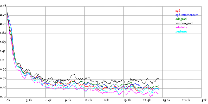
Karpathy做了一个这几个方法在MNIST上性能的比较，其结论是：
adagrad相比于sgd和momentum更加稳定，即不需要怎么调参。而精调的sgd和momentum系列方法无论是收敛速度还是precision都比adagrad要好一些。在精调参数下，一般Nesterov优于momentum优于sgd。而adagrad一方面不用怎么调参，另一方面其性能稳定优于其他方法。

实验结果图如下：

Loss vs. Number of examples seen

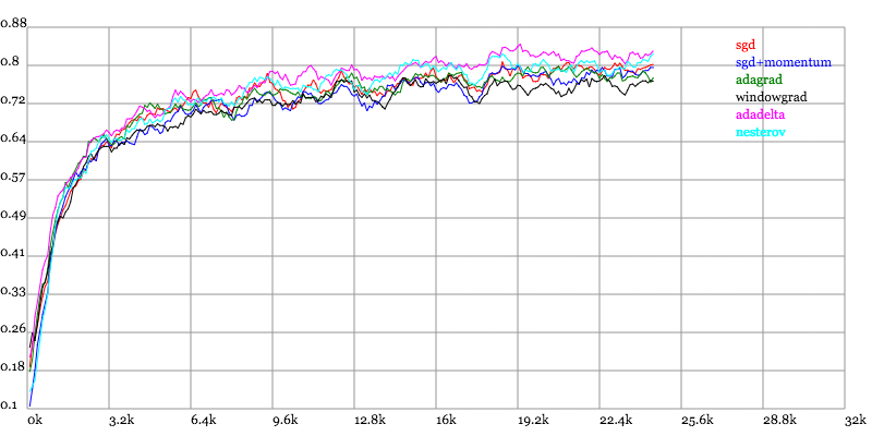
Testing Accuracy vs. Number of examples seen

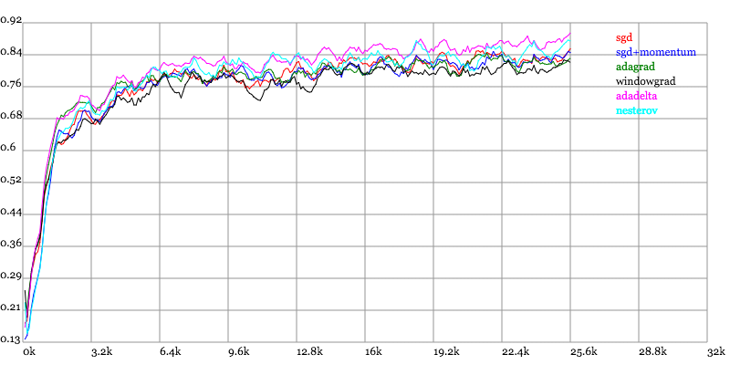
Training Accuracy vs. Number of examples seen