


一、PointRend理解
PointRend的提出是为了解决Mask RCNN分割精度不高的问题,个人建议想要学习这个网络的同学可以从语义分割模型上着手,毕竟Mask RCNN相比于语义分割模型还是比较复杂的,但是PointRend的思想是一样的。PoinRend语义分割
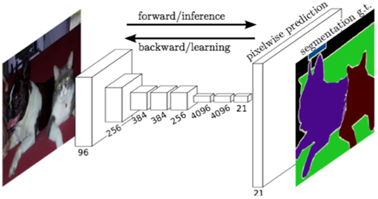
那么PointRend网络到底是如何解决分割结果精细度不高的问题呢?让我们来回顾一下语义分割领域最经典的FCN模型。
FCN语义分割思想:对原始图像经过不断的卷积和池化,得到高密度特征,然后直接上采样到与图像大小一致的结果,这样必然会导致分割结果很粗糙,尤其是边界部分误差很大。
之后大部分的语义分割模型都是基于这个框架来做的,只是在最后上采样部分做了修改,如Unet的decoder和deeplabV3+的decoder上采样。
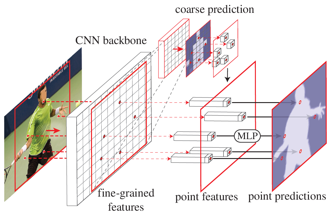
PointRend核心思想:语义分割经过多次池化降采样后,直接预测分类结果,而不是上采样到跟原图像同样尺寸。在粗糙的分割结果中选择分割精度不高的点,然后在这些点上结合粗糙和精细的特征训练MLP模型,对这些点进行重新预测,用重新预测的结果替换原来预测的粗糙结果。
1.1 语义分割模型训练
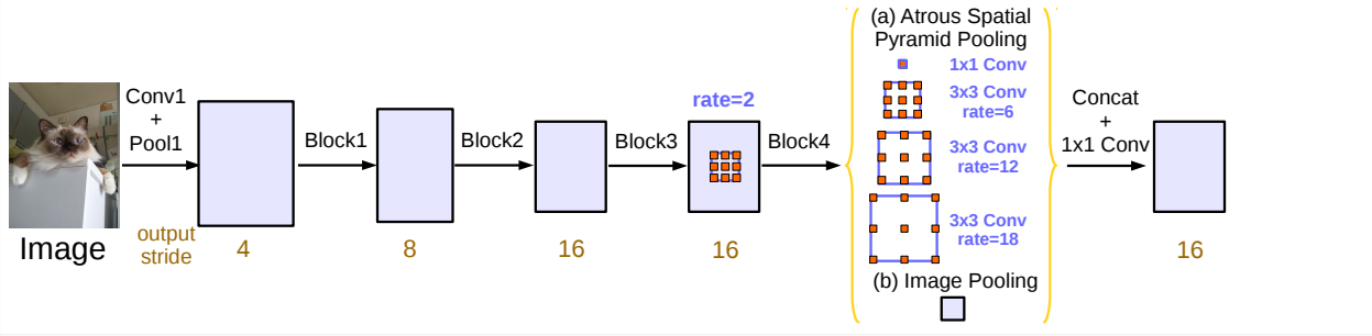
首先训练一个标准的语义分割网络训练(这里以deeplabv3为例),将上采样部分替换为3X3的卷积,最终层的通道数为分类数,把这个作为粗分割结果。如下图
1.2、选点
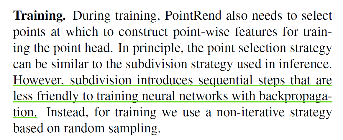
这一步的目的是选出N个点,然后对这N个点重新预测。选点策略在训练和推理的时候是不一样的。
训练时选点策略分三步
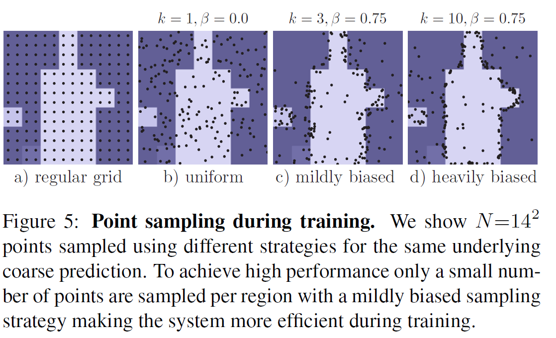
Over generation:随机生成k*N个点
Import sampling:选出最不确定的βN(β∈[0,1])个点。
Coverage:剩下的(1-β)N个点按照均匀分布的方式选择。
推理时选点的策略
每次先上采样2倍,然后直接选出不确定的N个点
1.3、特征提取
在精细特征图(deeplabV3中的res2输出结果)和粗糙特预测结果上提取步骤2中选出的N个点所在位置的特征,然后合并。
1.4、训练MLP,替换。
用上面提取特征作为样本训练一个MLP模型(实际实现是1x1卷积)。即可得到这些点重新预测的结果,在推理时,通过迭代上采样的方式逐步的替换这些精度不高的点,知道尺寸跟原图大小一致。
要点总结:训练和推理阶段的两处不同
1、选点策略不同
2、点替换策略不同
二、PointRend代码解释(为了节省空间,我删除了源码中大段的注释)
PointRend整体逻辑梳理
class PointRend(nn.Module):
    def __init__(self, backbone, head):
        super().__init__()
        self.backbone = backbone
        self.head = head

    def forward(self, x):
        result = self.backbone(x)
        result.update(self.head(x, result["res2"], result["coarse"]))
        return result
PointRend()类初始化就两部分,backbone和head。其中backbone就是deeplabv3,head是PointHead,即选择点重新训练的过程。重点在PointHead:
class PointHead(nn.Module):
    def __init__(self, in_c=533, num_classes=21, k=3, beta=0.75):
        super().__init__()
        self.mlp = nn.Conv1d(in_c, num_classes, 1)
        self.k = k
        self.beta = beta

    def forward(self, x, res2, out):
        if not self.training:
            return self.inference(x, res2, out)

        points = sampling_points(out, x.shape[-1] // 16, self.k, self.beta)

        coarse = point_sample(out, points, align_corners=False)
        fine = point_sample(res2, points, align_corners=False)

        feature_representation = torch.cat([coarse, fine], dim=1)

        rend = self.mlp(feature_representation)

        return {"rend": rend, "points": points}

    @torch.no_grad()
    def inference(self, x, res2, out):
        num_points = 8096

        while out.shape[-1] != x.shape[-1]:
            out = F.interpolate(out, scale_factor=2, mode="bilinear", align_corners=True)

            points_idx, points = sampling_points(out, num_points, training=self.training)

            coarse = point_sample(out, points, align_corners=False)
            fine = point_sample(res2, points, align_corners=False)

            feature_representation = torch.cat([coarse, fine], dim=1)

            rend = self.mlp(feature_representation)

            B, C, H, W = out.shape
            points_idx = points_idx.unsqueeze(1).expand(-1, C, -1)
            out = (out.reshape(B, C, -1)
                      .scatter_(2, points_idx, rend)
                      .view(B, C, H, W))

        return {"fine": out}
PointHead()类初始化有四个参数,in_c, num_classes, k=3, beta=0.75,超参数k和β,其中in_c是MLP的输入通道数,默认为533,这个数是咋来的呢,其实就是deeplabv3特征提取部分layer2输出特征层的通道数(512)+类别数(21)。
我们先来看训练阶段的前向传播过程
		#选点
        points = sampling_points(out, x.shape[-1] // 16, self.k, self.beta)

		#提取对应点上的特征
        coarse = point_sample(out, points, align_corners=False)
        fine = point_sample(res2, points, align_corners=False)
        feature_representation = torch.cat([coarse, fine], dim=1)
		#MLP
        rend = self.mlp(feature_representation)

        return {"rend": rend, "points": points}
分别对应1.2节的选点,1.3节的特征提取,1.4节的MLP训练。具体细节我们放在下面章节讲。
再看一下推理阶段的前向传播过程(通过training=False判断)
def inference(self, x, res2, out):
        num_points = 8096

        while out.shape[-1] != x.shape[-1]:
        	#上采样
            out = F.interpolate(out, scale_factor=2, mode="bilinear", align_corners=True)
			#选点
            points_idx, points = sampling_points(out, num_points, training=self.training)
			#特征提取
            coarse = point_sample(out, points, align_corners=False)
            fine = point_sample(res2, points, align_corners=False)

            feature_representation = torch.cat([coarse, fine], dim=1)
			#mlp预测
            rend = self.mlp(feature_representation)

            B, C, H, W = out.shape
            points_idx = points_idx.unsqueeze(1).expand(-1, C, -1)
            #替换采样点的分割结果
            out = (out.reshape(B, C, -1)
                      .scatter_(2, points_idx, rend)
                      .view(B, C, H, W))

        return {"fine": out}
deeplabV3输出的粗糙的分割结果每次上采样2倍,然后执行一次选点、特征提取、mlp预测的过程(跟训练时的流程一致,只是选点策略有区别),替换所选出的点上的分割结果,重复执行这个操作,直到分割结果的尺寸与原图尺寸大小一致。
这里有个问题,为啥PointRend的训练和推理的前向过程不一样呢?
2.1、选点策略
这一部分是选点的具体实现细节。
def sampling_points(mask, N, k=3, beta=0.75, training=True):
    assert mask.dim() == 4, "Dim must be N(Batch)CHW"
    device = mask.device
    B, _, H, W = mask.shape
    mask, _ = mask.sort(1, descending=True)

    if not training:
        H_step, W_step = 1 / H, 1 / W
        N = min(H * W, N)
        uncertainty_map = -1 * (mask[:, 0] - mask[:, 1])
        _, idx = uncertainty_map.view(B, -1).topk(N, dim=1)

        points = torch.zeros(B, N, 2, dtype=torch.float, device=device)
        points[:, :, 0] = W_step / 2.0 + (idx  % W).to(torch.float) * W_step
        points[:, :, 1] = H_step / 2.0 + (idx // W).to(torch.float) * H_step
        return idx, points

    over_generation = torch.rand(B, k * N, 2, device=device)
    over_generation_map = point_sample(mask, over_generation, align_corners=False)

    uncertainty_map = -1 * (over_generation_map[:, 0] - over_generation_map[:, 1])
    _, idx = uncertainty_map.topk(int(beta * N), -1)

    shift = (k * N) * torch.arange(B, dtype=torch.long, device=device)

    idx += shift[:, None]

    importance = over_generation.view(-1, 2)[idx.view(-1), :].view(B, int(beta * N), 2)
    coverage = torch.rand(B, N - int(beta * N), 2, device=device)
    return torch.cat([importance, coverage], 1).to(device)
可以看到推理和训练的选点策略是分开的,通过模型的training参数来判断当前是推理还是训练阶段。结合第1.2节介绍的选点策略,我们先来看训练阶段如何实现选点。
选点之前先对mask(deeplabV3 输出的粗糙分割结果)做了排序,这步的作用是为了确定所选点的不确定性大小,在选点的第二步会用到。
#在每个像素点上,对预测的每类得分按降序排序。
mask, _ = mask.sort(1, descending=True)
训练阶段选点第一步是Over generation,对应下面这两句代码:
    over_generation = torch.rand(B, k * N, 2, device=device)
    over_generation_map = point_sample(mask, over_generation, align_corners=False)
第一句很简单,就是随机生成 k*N 个二维坐标点,batch_size为B,所以随机生成的点的尺寸为[B,k*N,2]。
第二句调用了point_sample()函数,该函数实现如下:
def point_sample(input, point_coords, **kwargs):
    add_dim = False
    if point_coords.dim() == 3:
        add_dim = True
        point_coords = point_coords.unsqueeze(2)
    output = F.grid_sample(input, 2.0 * point_coords - 1.0, **kwargs)
    if add_dim:
        output = output.squeeze(3)
    return output
Point_sample()函数的核心是调用了torch的grid_sample()插值函数,主要是通过插值的方法获得指定点的值。
output = F.grid_sample(input, 2.0 * point_coords - 1.0, **kwargs)
先来看输入的参数,第一个参数input对应的是mask,也就是deeplabV3输出的粗糙的分割结果,第二个参数是要插值的点,输入的是2.0*point_coords-1.0,其中point_coords是之前随机生成的k*N (一张图片)个二维坐标点。那为啥要做一下这个线性变换呢?其实这是跟torch的grid_sample()原理有关。
grid_sample()输入的插值点的坐标是相对坐标,相对于mask的位置,其中左上角坐标是(-1,-1),右下角坐标是(1,1)。所以传入的坐标范围要在[-1,1]之间。具体原理可以另外一篇文章:PyTorch中grid_sample的使用方法。
从这里我们可以看到代码实现中所选的点坐标都是相对位置,这样才能将在不同尺寸的特征图上提取的特征合并。
然后是第二步:Import sampling,对应的代码如下
    uncertainty_map = -1 * (over_generation_map[:, 0] - over_generation_map[:, 1])
    _, idx = uncertainty_map.topk(int(beta * N), -1)

    shift = (k * N) * torch.arange(B, dtype=torch.long, device=device)

    idx += shift[:, None]

    importance = over_generation.view(-1, 2)[idx.view(-1), :].view(B, int(beta * N), 2)
这是很关键的一步操作,来逐句看一下是怎么实现的
    uncertainty_map = -1 * (over_generation_map[:, 0] - over_generation_map[:, 1])
    _, idx = uncertainty_map.topk(int(beta * N), -1)
第一类得分减去第二类得分(mask 已经在每个像素上按得分结果降序排列了),取反,然后取前β*N个点,就这?这样就取到了前β*N个最不确定的点?为啥要这么做呢?
我们来分析一下,我们知道1个像素点只对应1个类别,如果该像素对应的两个类别分数都很高或者说得分最高的两类分数很接近,说明它可能是边界点,也说明这个点的分割结果不确定性很高。
举个例子,假设分割任务有5类,像素A、B、C的分割得分如下表
| 像素点 | 1 | 2 | 3 | 4 | 5 | uncertain_map |
|---|---|---|---|---|---|---|
| A | 0.15 | 0.05 | 0.05 | 0.05 | 0.7 | -0.55 |
| B | 0.15 | 0.15 | 0.15 | 0.2 | 0.35 | -0.15 |
| C | 0.05 | 0.05 | 0.11 | 0.39 | 0.4 | -0.01 |
我们知道这三个像素都会被认定为是第5类,但是分类正确的可能性应该是A>B>C。我们按照代码中的不确定性计算方法得到uncertain_map_A=-0.55,uncertain_map_B=-0.15,uncertain_map_B=-0.01,明显uncertain_map_C要远大于uncertain_map_A和uncertain_map_B,因此在选点的时候,C会被选出来作为不确定性高的点。
第三步:Coverage,对应代码如下
coverage = torch.rand(B, N - int(beta * N), 2, device=device)
很简单,剩下的(1-β)*N个点随机生成即可。最后将importance点和coverage点合并返回即可。
return torch.cat([importance, coverage], 1).to(device)
然后我们再来看一下推理时如何选点。
    if not training:
        H_step, W_step = 1 / H, 1 / W
        N = min(H * W, N)
        uncertainty_map = -1 * (mask[:, 0] - mask[:, 1])
        _, idx = uncertainty_map.view(B, -1).topk(N, dim=1)

        points = torch.zeros(B, N, 2, dtype=torch.float, device=device)
        points[:, :, 0] = W_step / 2.0 + (idx  % W).to(torch.float) * W_step
        points[:, :, 1] = H_step / 2.0 + (idx // W).to(torch.float) * H_step
        return idx, points
与训练不同的是,推理时是直接选出N个不确定的点,点的不确定性的规则训练时一样。
注意:所选的点的坐标都是相对坐标
2.2、特征提取
2.1节获得了所需要的N个点,接下来就是获取这些点对应的精细层特征和粗糙层特征,用的方法也是torch的grid_sample()。代码如下
        coarse = point_sample(out, points, align_corners=False)
        fine = point_sample(res2, points, align_corners=False)

        feature_representation = torch.cat([coarse, fine], dim=1)
2.3、预测分类
得到所选的N个点的特征值之后,执行MLP操作,其实就是1X1的卷积。rend保存的就是这N个点新的分类结果。
rend = self.mlp(feature_representation)
其他
1、训练时如何计算loss
看train.py文件
        result = net(x)

        pred = F.interpolate(result["coarse"], x.shape[-2:], mode="bilinear", align_corners=True)
        seg_loss = F.cross_entropy(pred, gt, ignore_index=255)

        gt_points = point_sample(
            gt.float().unsqueeze(1),
            result["points"],
            mode="nearest",
            align_corners=False
        ).squeeze_(1).long()
        points_loss = F.cross_entropy(result["rend"], gt_points, ignore_index=255)

        loss = seg_loss + points_loss
net就是PoinRend网络,result为前向输出结果,里面包含了“coarse”,“points”,“rend”。
"coarse"即粗糙的分割结果,直接将其上采样到跟原图大小的结果(deeplabV3标准的最后一步操作),计算一次loss,即seg_loss;
“points”为选择的N个点,提取出这些点对应的真实值,即gt_points;
“rend”是MLP预测的N个点的结果,与gt_points计算一次loss,即points_loss。
2、推理的操作
在infer.py文件中,关键的就一句话
pred = net(x)["fine"].argmax(1)
推理前记得加上
net.eval()
这句是将网络中的training参数设置为False。
3、PointRend如何在Mask RCNN上使用
理解了一、二节介绍的PointRend网络在语义分割上使用的原理和实现细节后再来看PointRend如何在Mask Rcnn上使用应该会简单很多了。
其实还是backbone和pointHead,只不过backbone不一样了。(这里假定大家已经了解了Mask RCNN的原理)。
来看一下PointRend原文里给的结构图


 7069
7069

 被折叠的 条评论
为什么被折叠?
被折叠的 条评论
为什么被折叠?
 到【灌水乐园】发言


