


MVSNet通过将相机几何参数编码到网络中,实现了端到端的多视角三维重建,并在性能和视觉效果上超越了先前算法,并在eccv2018 oral中发表。
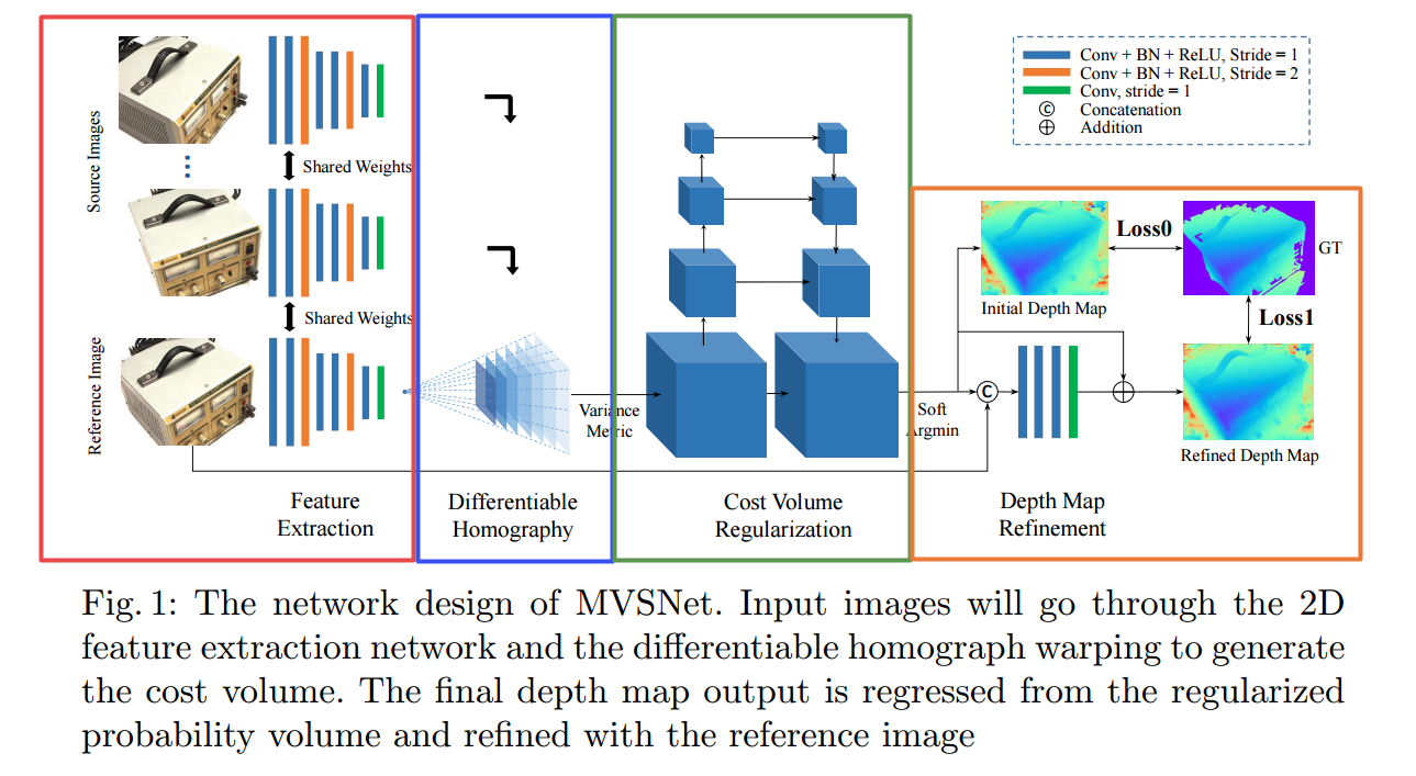
模型主要包含四个主要步骤:图像特征抽取、多视角可微单应性变换、cost volume构建和正则化、深度估计与深度优化。更多算法和实现过程中的细节分析,请参看代码MVSNet的 ? 论文解读
其代码使用tensorflow实现,包含了训练和测试模块,由Yaoyao开发。
MVSNet
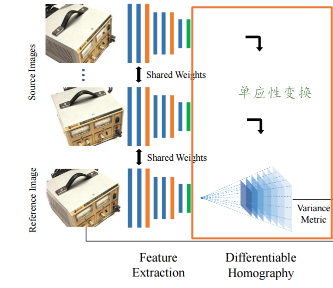
首先回顾一下MVSNet的目标任务和模型结构,其任务是通过对视角图像重建出目标的三维表示。
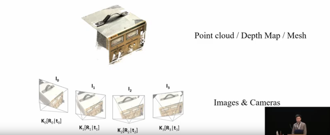
其模型结构包含了四个部分,分别是特征抽取、单应性变换、代价空间构造和深度图估计与优化。它的主要贡献在与三个方面:
- 一是利用可微的单应性变换将多个参考视图的图像特征变换到了参考图像视角下的不同深度上,并基于此构建cost volume实现了端到端的训练;
- 二是将三维重建问题分解为了对应视角下的深度估计问题,使得大规模的多视角三维重建成为可能;
- 三是利用基于方差的cost metric实现了对于任意视角图像数量的有效处理。
2.代码结构分析
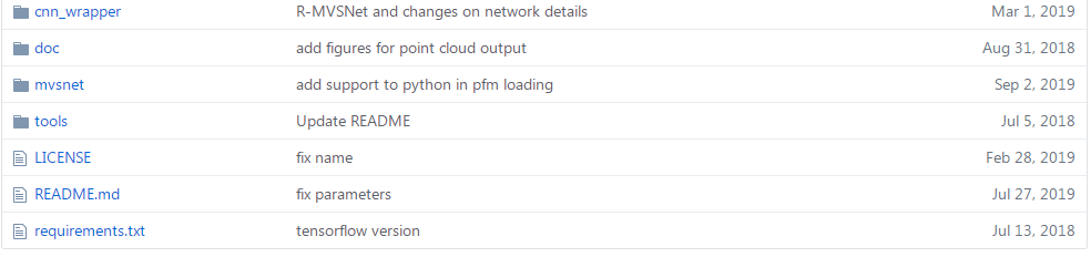
这一工作对应的源码主要包含了以下仨个文件夹,其中mvsnet/为网络的实现训练测试部分,tools/common.py内部包含了各种工具函数,cnn_warpper/network.py mvsnet.py则包含了各种cnn操作和子模块实现函数:
如果要快速上手使用可以在下载代码配置好后运行:
cd MVSNet/mvsnet
python train.py --regularization '3DCNNs'
? 我们先来分析训练代码MVSNet/mvsnet/train.py的构造:
# copy from https://github.com/YoYo000/MVSNet/blob/master/mvsnet/train.py
# 省略各种import和初始化参数设置
# 其中包含了生成训练数据的class MVSGenerator:
# 计算梯度的:def average_gradients(tower_grads):
# 进行训练的函数:def train(traning_list):


###---------------------------------------------------------------------###
# 首先来看如何构造出整个模型
class MVSGenerator:
    """ data generator class, tf only accept generator without param """
    def __init__(self, sample_list, view_num):
        self.sample_list = sample_list     # 样本标
        self.view_num = view_num           # MVS中视角的数目
        self.sample_num = len(sample_list) # 样本数量
        self.counter = 0                   # 计数器

    def __iter__(self):
        while True:
            for data in self.sample_list:
                start_time = time.time()

                ###### read input data ######
                # 读入数据,包含图像和相机参数,以及对应的GT深度图
                images = []
                cams = []
                for view in range(self.view_num):
                    image = center_image(cv2.imread(data[2 * view]))
                    cam = load_cam(open(data[2 * view + 1]))
                    cam[1][3][1] = cam[1][3][1] * FLAGS.interval_scale  #下采样尺度
                    images.append(image)
                    cams.append(cam)
                depth_image = load_pfm(open(data[2 * self.view_num]))

                # mask out-of-range depth pixels (in a relaxed range)
                # 训练过程中深度设定在一个范围内,
                depth_start = cams[0][1, 3, 0] + cams[0][1, 3, 1]
                depth_end = cams[0][1, 3, 0] + (FLAGS.max_d - 2) * cams[0][1, 3, 1]
                depth_image = mask_depth_image(depth_image, depth_start, depth_end)

                # return mvs input
                self.counter += 1
                duration = time.time() - start_time
                images = np.stack(images, axis=0)
                cams = np.stack(cams, axis=0)
                #max_d为训练的最大深度step值
                print('Forward pass: d_min = %f, d_max = %f.' % \
                    (cams[0][1, 3, 0], cams[0][1, 3, 0] + (FLAGS.max_d - 1) * cams[0][1, 3, 1]))
                yield (images, cams, depth_image)    # ---->返回生成的训练数据包括图像 相机参数和对应深度图

                # return backward mvs input for GRU
                # 这里是为R-MVSNet设计的新入口 后续文章分析
                if FLAGS.regularization == 'GRU':
                    self.counter += 1
                    start_time = time.time()
                    cams[0][1, 3, 0] = cams[0][1, 3, 0] + (FLAGS.max_d - 1) * cams[0][1, 3, 1]
                    cams[0][1, 3, 1] = -cams[0][1, 3, 1]
                    duration = time.time() - start_time
                    print('Back pass: d_min = %f, d_max = %f.' % \
                        (cams[0][1, 3, 0], cams[0][1, 3, 0] + (FLAGS.max_d - 1) * cams[0][1, 3, 1]))
                    yield (images, cams, depth_image)


###---------------------------------------------------------------------###
# 计算梯度 这里定义了多个不同GPU间的进行传递 和梯度平均
# 针对单GPU的大多数小伙伴来说基本可以忽略
def average_gradients(tower_grads):
    """Calculate the average gradient for each shared variable across all towers.
    Note that this function provides a synchronization point across all towers.
    Args:
    tower_grads: List of lists of (gradient, variable) tuples. The outer list
        is over individual gradients. The inner list is over the gradient
        calculation for each tower.
    Returns:
        List of pairs of (gradient, variable) where the gradient has been averaged
        across all towers.
    """
    average_grads = []
    for grad_and_vars in zip(*tower_grads):
        # Note that each grad_and_vars looks like the following:
        #   ((grad0_gpu0, var0_gpu0), ... , (grad0_gpuN, var0_gpuN))
        grads = []
        for g, _ in grad_and_vars:
            # Add 0 dimension to the gradients to represent the tower.
            expanded_g = tf.expand_dims(g, 0)

            # Append on a 'tower' dimension which we will average over below.
            grads.append(expanded_g)

        # Average over the 'tower' dimension.
        grad = tf.concat(axis=0, values=grads)
        grad = tf.reduce_mean(grad, 0)

        # Keep in mind that the Variables are redundant because they are shared
        # across towers. So .. we will just return the first tower's pointer to
        # the Variable.
        # 共享 指向第一GPU的指针 变量是共享的 同时使用平均后的grad梯度
        v = grad_and_vars[0][1]
        grad_and_var = (grad, v)
        average_grads.append(grad_and_var)
    return average_grads


###------------------------------------------------------------------------###
# 训练代码
# 其中包含了载入预训练模型的部分和GRU部分的代码暂时省略

def train(traning_list):
    """ training mvsnet """
    training_sample_size = len(traning_list)
    if FLAGS.regularization == 'GRU':     # GRU R-MVSNet的部分
        training_sample_size = training_sample_size * 2
    print ('sample number: ', training_sample_size)

    with tf.Graph().as_default(), tf.device('/cpu:0'):    # 默认CPU

        ########## data iterator #########
        # 生成数据迭代器
        # training generators
        training_generator = iter(MVSGenerator(traning_list, FLAGS.view_num))
        generator_data_type = (tf.float32, tf.float32, tf.float32)
        # dataset from generator
        training_set = tf.data.Dataset.from_generator(lambda: training_generator, generator_data_type)
        training_set = training_set.batch(FLAGS.batch_size)
        training_set = training_set.prefetch(buffer_size=1)
        # iterators
        training_iterator = training_set.make_initializable_iterator()

        ########## optimization options ##########
        # 优化参数设计,学习率衰减  使用RMSPropOtimizer作为优化器
        global_step = tf.Variable(0, trainable=False, name='global_step')
        lr_op = tf.train.exponential_decay(FLAGS.base_lr, global_step=global_step,
                                           decay_steps=FLAGS.stepvalue, decay_rate=FLAGS.gamma, name='lr')
        opt = tf.train.RMSPropOptimizer(learning_rate=lr_op)

        tower_grads = []
        for i in xrange(FLAGS.num_gpus):  # 多个GPU上循环
            with tf.device('/gpu:%d' % i):
                with tf.name_scope('Model_tower%d' % i) as scope:
                    # generate data   生成数据,包括输入的多视角图像和相机参数 loss处使用的深度图
                    images, cams, depth_image = training_iterator.get_next()
                    images.set_shape(tf.TensorShape([None, FLAGS.view_num, None, None, 3]))
                    cams.set_shape(tf.TensorShape([None, FLAGS.view_num, 2, 4, 4]))
                    depth_image.set_shape(tf.TensorShape([None, None, None, 1]))
                    depth_start = tf.reshape(
                        tf.slice(cams, [0, 0, 1, 3, 0], [FLAGS.batch_size, 1, 1, 1, 1]), [FLAGS.batch_size])
                    depth_interval = tf.reshape(
                        tf.slice(cams, [0, 0, 1, 3, 1], [FLAGS.batch_size, 1, 1, 1, 1]), [FLAGS.batch_size])

                    is_master_gpu = False
                    if i == 0:
                        is_master_gpu = True

                    # inference
                    if FLAGS.regularization == '3DCNNs':
                    # 训练基于3DCNN的cost volume regular
                    # 主要包含了初始深度图inference 和最后深度图的depth_refine 以及loss计算
                        # initial depth map
                        # 这里的inference函数来自于model.py中
                        depth_map, prob_map = inference(
                            images, cams, FLAGS.max_d, depth_start, depth_interval, is_master_gpu)

                        # refinement
                        if FLAGS.refinement:
                            ref_image = tf.squeeze(
                                tf.slice(images, [0, 0, 0, 0, 0], [-1, 1, -1, -1, 3]), axis=1)
                            refined_depth_map = depth_refine(depth_map, ref_image,
                                    FLAGS.max_d, depth_start, depth_interval, is_master_gpu)
                        else:
                            refined_depth_map = depth_map

                        # regression loss
                        # 计算两个损失ff
                        loss0, less_one_temp, less_three_temp = mvsnet_regression_loss(
                            depth_map, depth_image, depth_interval)
                        loss1, less_one_accuracy, less_three_accuracy = mvsnet_regression_loss(
                            refined_depth_map, depth_image, depth_interval)
                        loss = (loss0 + loss1) / 2

        # 省略各种tensorboard的记录和日志


###----------------------------------------------------------###
# session训练过程
        with tf.Session(config=config) as sess:

            # initialization
            total_step = 0
            sess.run(init_op)
            summary_writer = tf.summary.FileWriter(FLAGS.log_dir, sess.graph)

            # load pre-trained model
            # 省略载入预训练模型

            # training several epochs
            for epoch in range(FLAGS.epoch):

                # training of one epoch
                step = 0
                sess.run(training_iterator.initializer)
                for _ in range(int(training_sample_size / FLAGS.num_gpus)):

                    # run one batch
                    start_time = time.time()
                    # 计算损失函数 包括深度估计损失 各种日志和重投影误差等
                    try:
                        out_summary_op, out_opt, out_loss, out_less_one, out_less_three = sess.run(
                        [summary_op, train_opt, loss, less_one_accuracy, less_three_accuracy])
                    except tf.errors.OutOfRangeError:
                        print("End of dataset")  # ==> "End of dataset"
                        break
                    duration = time.time() - start_time

                    # print info
                    if step % FLAGS.display == 0:
                        print(Notify.INFO,
                            'epoch, %d, step %d, total_step %d, loss = %.4f, (< 1px) = %.4f, (< 3px) = %.4f (%.3f sec/step)' %
                            (epoch, step, total_step, out_loss, out_less_one, out_less_three, duration), Notify.ENDC)

                    # write summary
                    if step % (FLAGS.display * 10) == 0:
                        summary_writer.add_summary(out_summary_op, total_step)

                    # save the model checkpoint periodically
                    # 保存模型
                    if (total_step % FLAGS.snapshot == 0 or step == (training_sample_size - 1)):
                        model_folder = os.path.join(FLAGS.model_dir, FLAGS.regularization)
                        if not os.path.exists(model_folder):
                            os.mkdir(model_folder)
                        ckpt_path = os.path.join(model_folder, 'model.ckpt')
                        print(Notify.INFO, 'Saving model to %s' % ckpt_path, Notify.ENDC)
                        saver.save(sess, ckpt_path, global_step=total_step)
                    step += FLAGS.batch_size * FLAGS.num_gpus
                    total_step += FLAGS.batch_size * FLAGS.num_gpus
?其中的主要操作是来自与model.py的函数,包括inference 和depth_refine以及计算损失的mvsnet_regression_loss,下面我们分别来分析这三个函数:
# inference()
# 其中还包含了额外三个初始深度估计的函数,用于R-MVSNet论文中的方法比较:
#      inference_mem() inference_prob_recurrent()  inference_winner_take_all()
# copy from https://github.com/YoYo000/MVSNet/blob/master/mvsnet/model.py
#
#
# 其主要过程是提取图像特征,将图像特征进行单应性变换,组成代价空间,并基于代价空间估计深度

def inference(images, cams, depth_num, depth_start, depth_interval, is_master_gpu=True):
    """ infer depth image from multi-view images and cameras """

    # dynamic gpu params
    depth_end = depth_start + (tf.cast(depth_num, tf.float32) - 1) * depth_interval

    # reference image
    # 参考图像的特征抽取
    ref_image = tf.squeeze(tf.slice(images, [0, 0, 0, 0, 0], [-1, 1, -1, -1, 3]), axis=1)
    ref_cam = tf.squeeze(tf.slice(cams, [0, 0, 0, 0, 0], [-1, 1, 2, 4, 4]), axis=1)

    # image feature extraction
    if is_master_gpu:
        ref_tower = UNetDS2GN({'data': ref_image}, is_training=True, reuse=False)
    else:
        ref_tower = UNetDS2GN({'data': ref_image}, is_training=True, reuse=True)
    view_towers = []
    # 多视角图像的特征抽取
    for view in range(1, FLAGS.view_num):
        view_image = tf.squeeze(tf.slice(images, [0, view, 0, 0, 0], [-1, 1, -1, -1, -1]), axis=1)
        view_tower = UNetDS2GN({'data': view_image}, is_training=True, reuse=True)
        view_towers.append(view_tower)

    # get all homographies
    # 获取多视角图像相对于参考图像的单应性变换矩阵计算
    view_homographies = []
    for view in range(1, FLAGS.view_num):
        view_cam = tf.squeeze(tf.slice(cams, [0, view, 0, 0, 0], [-1, 1, 2, 4, 4]), axis=1)
        homographies = get_homographies(ref_cam, view_cam, depth_num=depth_num,
                                        depth_start=depth_start, depth_interval=depth_interval)
        view_homographies.append(homographies)

    # build cost volume by differentialble homography
    # 计算每个深度上的cost 对应论文中3.2第二部分
    with tf.name_scope('cost_volume_homography'):
        depth_costs = []
        # 两层循环,外层是参考视角下多个深度di上,内层是每个视角都要变换到参考视角的给定深度下
        for d in range(depth_num):
            # compute cost (variation metric)
            ave_feature = ref_tower.get_output()
            ave_feature2 = tf.square(ref_tower.get_output())
            for view in range(0, FLAGS.view_num - 1):
                homography = tf.slice(view_homographies[view], begin=[0, d, 0, 0], size=[-1, 1, 3, 3])
                homography = tf.squeeze(homography, axis=1)
                # 进行单应性变换,并将每次变换后的特征加在对应深度上
				# warped_view_feature = homography_warping(view_towers[view].get_output(), homography)
                warped_view_feature = tf_transform_homography(view_towers[view].get_output(), homography)
                ave_feature = ave_feature + warped_view_feature
                ave_feature2 = ave_feature2 + tf.square(warped_view_feature)
            ave_feature = ave_feature / FLAGS.view_num
            ave_feature2 = ave_feature2 / FLAGS.view_num
            cost = ave_feature2 - tf.square(ave_feature)
            depth_costs.append(cost)
        cost_volume = tf.stack(depth_costs, axis=1)

    # filtered cost volume, size of (B, D, H, W, 1)
    # 利用多尺度3DCNN来对代价空间进行正则化,是一个四个尺度的UNet
    if is_master_gpu:
        filtered_cost_volume_tower = RegNetUS0({'data': cost_volume}, is_training=True, reuse=False)
    else:
        filtered_cost_volume_tower = RegNetUS0({'data': cost_volume}, is_training=True, reuse=True)
    filtered_cost_volume = tf.squeeze(filtered_cost_volume_tower.get_output(), axis=-1)

    # depth map by softArgmin
    # 最后利用softmax 沿着深度方向来直接获取概率归一化结果--->得到概率体积probability volume
    # 1.计算深度期望
    # 2.计算概率分布评价深度生成质量
    with tf.name_scope('soft_arg_min'):
        # probability volume by soft max
        probability_volume = tf.nn.softmax(
            tf.scalar_mul(-1, filtered_cost_volume), axis=1, name='prob_volume')
        # depth image by soft argmin
        volume_shape = tf.shape(probability_volume)
        soft_2d = []
        for i in range(FLAGS.batch_size):
            soft_1d = tf.linspace(depth_start[i], depth_end[i], tf.cast(depth_num, tf.int32))
            soft_2d.append(soft_1d)
        soft_2d = tf.reshape(tf.stack(soft_2d, axis=0), [volume_shape[0], volume_shape[1], 1, 1])
        soft_4d = tf.tile(soft_2d, [1, 1, volume_shape[2], volume_shape[3]])
        estimated_depth_map = tf.reduce_sum(soft_4d * probability_volume, axis=1)
        estimated_depth_map = tf.expand_dims(estimated_depth_map, axis=3)

    # probability map
    prob_map = get_propability_map(probability_volume, estimated_depth_map, depth_start, depth_interval)

    return estimated_depth_map, prob_map#, filtered_depth_map, probability_volume
?紧接着需要对上一步基于概率volume得到的深度进行refine。由于在正则化阶段较大的感受野使得重建的边缘过于平滑,这就需要从参考图像中获取边缘信息来优化这些区域的精度。优化阶段使用了深度残差网络来进行,输入为上一步估计的初始深度+参考图像的4通道,通过三个32通道的二维卷积和一个单通道的卷积(最后一层输出残差,不加激活和BN),并与初始深度相加得到优化后的深度(为了避免深度的尺度效应,统一归一化到0-1而后又在优化后重新计算回来)。
# copy from https://github.com/YoYo000/MVSNet/blob/master/mvsnet/model.py
# 主要对深度和参考图像进行边缘信息提取 利用残差优化初始深度图的边缘区域精度

def depth_refine(init_depth_map, image, depth_num, depth_start, depth_interval, is_master_gpu=True):
    """ refine depth image with the image
    先对深度图进行归一化
    再对参考图像进行尺度缩放1/4
    再利用残差网络计算残差
    最后恢复正常深度
    """

    # normalization parameters
    depth_shape = tf.shape(init_depth_map)
    depth_end = depth_start + (tf.cast(depth_num, tf.float32) - 1) * depth_interval
    depth_start_mat = tf.tile(tf.reshape(
        depth_start, [depth_shape[0], 1, 1, 1]), [1, depth_shape[1], depth_shape[2], 1])
    depth_end_mat = tf.tile(tf.reshape(
        depth_end, [depth_shape[0], 1, 1, 1]), [1, depth_shape[1], depth_shape[2], 1])
    depth_scale_mat = depth_end_mat - depth_start_mat

    # normalize depth map (to 0~1)
    init_norm_depth_map = tf.div(init_depth_map - depth_start_mat, depth_scale_mat)

    # resize normalized image to the same size of depth image
    resized_image = tf.image.resize_bilinear(image, [depth_shape[1], depth_shape[2]])

    # refinement network
    if is_master_gpu:
        norm_depth_tower = RefineNet({'color_image': resized_image, 'depth_image': init_norm_depth_map},
                                        is_training=True, reuse=False)
    else:
        norm_depth_tower = RefineNet({'color_image': resized_image, 'depth_image': init_norm_depth_map},
                                        is_training=True, reuse=True)
    norm_depth_map = norm_depth_tower.get_output()

    # denormalize depth map
    refined_depth_map = tf.multiply(norm_depth_map, depth_scale_mat) + depth_start_mat

    return refined_depth_map

# 其中RfineNet在子函数打包的函数cnn_wrapper/mvsnet.py中实现
class RefineNet(Network):
    """network for depth map refinement using original image."""

    def setup(self):
        # 输入四通道
        (self.feed('color_image', 'depth_image')
        .concat(axis=3, name='concat_image'))

        # 三个32卷积一个1通道卷积没有激活和BN
        # 输出直接为深度优化的残差
        (self.feed('concat_image')
        .conv_bn(3, 32, 1, name='refine_conv0')
        .conv_bn(3, 32, 1, name='refine_conv1')
        .conv_bn(3, 32, 1, name='refine_conv2')
        .conv(3, 1, 1, relu=False, name='refine_conv3'))

        # 与原深度图相加得到最终优化后的深度图
        (self.feed('refine_conv3', 'depth_image')
        .add(name='refined_depth_image'))
?最后我们来一起看一下整个模型的损失函数mvsnet/loss.py,包括初始深度损失和优化后的深度损失两部分,这两部分都仅仅对于基准图像中存在的点进行计算,λ取值为1:
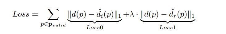
# 在训练代码中 计算损失为mvsnet_regression_loss() 并且只使用了三个返回值中的第一个mae值
# mvsnet/train.py line231
# regression loss
loss0, less_one_temp, less_three_temp = mvsnet_regression_loss(
    depth_map, depth_image, depth_interval)
loss1, less_one_accuracy, less_three_accuracy = mvsnet_regression_loss(
    refined_depth_map, depth_image, depth_interval)
loss = (loss0 + loss1) / 2

# 损失函数的具体定义 mvsnet/loss.py  mvsnet_regression_loss()
def mvsnet_regression_loss(estimated_depth_image, depth_image, depth_interval):
    """ compute loss and accuracy """
    # non zero mean absulote loss
    masked_mae = non_zero_mean_absolute_diff(depth_image, estimated_depth_image, depth_interval)
    # less one accuracy 误差小于1的点的精度
    less_one_accuracy = less_one_percentage(depth_image, estimated_depth_image, depth_interval)
    # less three accuracy  误差小于3的点的精度
    less_three_accuracy = less_three_percentage(depth_image, estimated_depth_image, depth_interval)

    return masked_mae, less_one_accuracy, less_three_accuracy


##------------------------------------------>>>>>>>>
# 其中包含了三个损失,主要使用了第一个非零位置的mae值
def non_zero_mean_absolute_diff(y_true, y_pred, interval):
    """ non zero mean absolute loss for one batch """
    with tf.name_scope('MAE'):
        shape = tf.shape(y_pred)
        interval = tf.reshape(interval, [shape[0]])
        mask_true = tf.cast(tf.not_equal(y_true, 0.0), dtype='float32')    # 获取非零位置掩膜
        denom = tf.reduce_sum(mask_true, axis=[1, 2, 3]) + 1e-7            # 计算非零值数量 作为均值的分母
        masked_abs_error = tf.abs(mask_true * (y_true - y_pred))            # 4D
        masked_mae = tf.reduce_sum(masked_abs_error, axis=[1, 2, 3])        # 1D
        masked_mae = tf.reduce_sum((masked_mae / interval) / denom)         # 1   对不同深度depth和非零值求均值
    return masked_mae

##------------------------------------------>>>>>>>>
# 第二个less_one_percentage()
def less_one_percentage(y_true, y_pred, interval):
    """ less one accuracy for one batch """
    with tf.name_scope('less_one_error'):
        shape = tf.shape(y_pred)
        mask_true = tf.cast(tf.not_equal(y_true, 0.0), dtype='float32')
        denom = tf.reduce_sum(mask_true) + 1e-7
        interval_image = tf.tile(tf.reshape(interval, [shape[0], 1, 1, 1]), [1, shape[1], shape[2], 1])
        abs_diff_image = tf.abs(y_true - y_pred) / interval_image  # 在深度上求均值
        # 计算误差小于1的值的损失mae
        less_one_image = mask_true * tf.cast(tf.less_equal(abs_diff_image, 1.0), dtype='float32')
    return tf.reduce_sum(less_one_image) / denom

##------------------------------------------>>>>>>>>
# 第三个less_three_percentage()
def less_three_percentage(y_true, y_pred, interval):
    """ less three accuracy for one batch """
    with tf.name_scope('less_three_error'):
        shape = tf.shape(y_pred)
        mask_true = tf.cast(tf.not_equal(y_true, 0.0), dtype='float32')
        denom = tf.reduce_sum(mask_true) + 1e-7
        interval_image = tf.tile(tf.reshape(interval, [shape[0], 1, 1, 1]), [1, shape[1], shape[2], 1])
        abs_diff_image = tf.abs(y_true - y_pred) / interval_image   # 在深度上求均值
        # 计算误差小于3的值的损失mae
        less_three_image = mask_true * tf.cast(tf.less_equal(abs_diff_image, 3.0), dtype='float32')
    return tf.reduce_sum(less_three_image) / denom
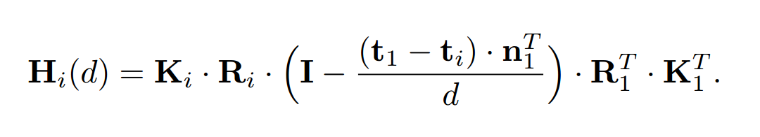
3.可微单应性变换
整篇文章的核心在于可微的单应性变换,将不同视角下图像特征转化到参考图像视角下的不同深度上去。
将第i个视角的特征Fi变换到对应深度的Vi(d)上去需要计算单应性变换矩阵Hi(d):
在前面的model.py中已经在inference()有过使用,具体是mvsnet/homography_warping.py中的get_homographies & tf_transform_homography两个函数:
# copy from https://github.com/YoYo000/MVSNet/blob/master/mvsnet/homography_warping.py
# 首先需要根据上面公式针对参考图像和多视角图像计算对应的变换矩阵
# left right对应了参考图像1和多视角图像i
# 相见论文3.3第二部分

def get_homographies(left_cam, right_cam, depth_num, depth_start, depth_interval):
    with tf.name_scope('get_homographies'):
        # cameras (K, R, t) 内参和外参
        R_left = tf.slice(left_cam, [0, 0, 0, 0], [-1, 1, 3, 3])
        R_right = tf.slice(right_cam, [0, 0, 0, 0], [-1, 1, 3, 3])
        t_left = tf.slice(left_cam, [0, 0, 0, 3], [-1, 1, 3, 1])
        t_right = tf.slice(right_cam, [0, 0, 0, 3], [-1, 1, 3, 1])
        K_left = tf.slice(left_cam, [0, 1, 0, 0], [-1, 1, 3, 3])
        K_right = tf.slice(right_cam, [0, 1, 0, 0], [-1, 1, 3, 3])

        # depth 深度采样
        depth_num = tf.reshape(tf.cast(depth_num, 'int32'), [])
        depth = depth_start + tf.cast(tf.range(depth_num), tf.float32) * depth_interval
        # preparation 预处理 左右相机left right
        num_depth = tf.shape(depth)[0]
        K_left_inv = tf.matrix_inverse(tf.squeeze(K_left, axis=1))
        R_left_trans = tf.transpose(tf.squeeze(R_left, axis=1), perm=[0, 2, 1])
        R_right_trans = tf.transpose(tf.squeeze(R_right, axis=1), perm=[0, 2, 1])

        # 左相机作为参考
        fronto_direction = tf.slice(tf.squeeze(R_left, axis=1), [0, 2, 0], [-1, 1, 3])          # (B, D, 1, 3)

        # 外参的trans  相对误差
        c_left = -tf.matmul(R_left_trans, tf.squeeze(t_left, axis=1))
        c_right = -tf.matmul(R_right_trans, tf.squeeze(t_right, axis=1))                        # (B, D, 3, 1)
        c_relative = tf.subtract(c_right, c_left)

        # compute   相对差与主相机方向相乘(t1-ti)·n1T  其中n1为参考相机方向
        batch_size = tf.shape(R_left)[0]
        temp_vec = tf.matmul(c_relative, fronto_direction)
        depth_mat = tf.tile(tf.reshape(depth, [batch_size, num_depth, 1, 1]), [1, 1, 3, 3])  # tile平铺

        temp_vec = tf.tile(tf.expand_dims(temp_vec, axis=1), [1, num_depth, 1, 1])

        # 中间括号里的计算 (I - (t1-ti)·n1T./d)--->((I - temp_vec/d))
        middle_mat0 = tf.eye(3, batch_shape=[batch_size, num_depth]) - temp_vec / depth_mat
        # 后半部分乘积()·R1·K1
        middle_mat1 = tf.tile(tf.expand_dims(tf.matmul(R_left_trans, K_left_inv), axis=1), [1, num_depth, 1, 1])
        middle_mat2 = tf.matmul(middle_mat0, middle_mat1)

        # 左半部分乘积Ki·Ri·()
        homographies = tf.matmul(tf.tile(K_right, [1, num_depth, 1, 1])
                     , tf.matmul(tf.tile(R_right, [1, num_depth, 1, 1])
                     , middle_mat2))


# 此时得到了某个视角下的特征图 向参考视角下多个深度进行变换的单应性矩阵
# 基于homography下一步就可以对特征向对应深度上进行变换了
# homography = tf.slice(view_homographies[view], begin=[0, d, 0, 0], size=[-1, 1, 3, 3])
# warped_view_feature = tf_transform_homography(view_towers[view].get_output(), homography)
###----------------------------------------------------------------------------###
def tf_transform_homography(input_image, homography):
    # 从图像坐标转到像素坐标以便使用tf.*.transform(),重新计算单应性矩阵
	# tf.contrib.image.transform is for pixel coordinate but our
	# homograph parameters are for image coordinate (x_p = x_i + 0.5).
	# So need to change the corresponding homography parameters
    homography = tf.reshape(homography, [-1, 9])
    a0 = tf.slice(homography, [0, 0], [-1, 1])
    a1 = tf.slice(homography, [0, 1], [-1, 1])
    a2 = tf.slice(homography, [0, 2], [-1, 1])
    b0 = tf.slice(homography, [0, 3], [-1, 1])
    b1 = tf.slice(homography, [0, 4], [-1, 1])
    b2 = tf.slice(homography, [0, 5], [-1, 1])
    c0 = tf.slice(homography, [0, 6], [-1, 1])
    c1 = tf.slice(homography, [0, 7], [-1, 1])
    c2 = tf.slice(homography, [0, 8], [-1, 1])
    a_0 = a0 - c0 / 2
    a_1 = a1 - c1 / 2
    a_2 = (a0 + a1) / 2 + a2 - (c0 + c1) / 4 - c2 / 2
    b_0 = b0 - c0 / 2
    b_1 = b1 - c1 / 2
    b_2 = (b0 + b1) / 2 + b2 - (c0 + c1) / 4 - c2 / 2
    c_0 = c0
    c_1 = c1
    c_2 = c2 + (c0 + c1) / 2
    homo = []
    homo.append(a_0)
    homo.append(a_1)
    homo.append(a_2)
    homo.append(b_0)
    homo.append(b_1)
    homo.append(b_2)
    homo.append(c_0)
    homo.append(c_1)
    homo.append(c_2)
    homography = tf.stack(homo, axis=1)
    homography = tf.reshape(homography, [-1, 9])

    homography_linear = tf.slice(homography, begin=[0, 0], size=[-1, 8])
    homography_linear_div = tf.tile(tf.slice(homography, begin=[0, 8], size=[-1, 1]), [1, 8])
    homography_linear = tf.div(homography_linear, homography_linear_div)  # 前八个元素进行归一化
    warped_image = tf.contrib.image.transform(
        input_image, homography_linear, interpolation='BILINEAR')   #可差分的过程

    # return input_image 得到变换后结果
    return warped_image

# 还有一个是homography_warping()函数 作者自己实现了变换过程及其需要的可差分插值函数 可以参考同一个代码实现
?最后详细说明一下几个重要的函数,其中打包了模型的基础操作子、子函数和IO等。
cnn_wrapper/network.py:包含了基本的NetWork基类,其中实现了conv cov_bn conv_gn deconv deconv_bn deconv_gn等基本卷积操作和max avg l2一系列池化、输出输出、加和衔接等操作;
cnn_wrapper/mvsnet.py:包含了基于Network基类构建的各种子网络模块,用于2D特征提取的的UniNet UNet,用于构建代价空间正则的RegNetUS0,用于得到深度残差进行优化的RefineNet等;
mvsnet/colmap2mvsnet.py:负责读入模型,相机参数、图像、点云等等I/O操作;
mvsnet/visualize.py:基于matplotlib的可视化操作;
mvsnet/depthfusion.py:转换为可以Gipuma处理的格式;
mvsnet/preprocess.py:各种载入点云数据集和相机参数,格式化前处理过程。
更多算法和实现过程中的细节分析,请参看MVSNet的 [ ? 论文解读]


 1297
1297


 被折叠的 条评论
为什么被折叠?
被折叠的 条评论
为什么被折叠?
 到【灌水乐园】发言


