一维信号光滑去毛刺处理

  以下是威斯康星大学交通系博士申请遇到的一道题，有兴趣的可以交流

Problem：

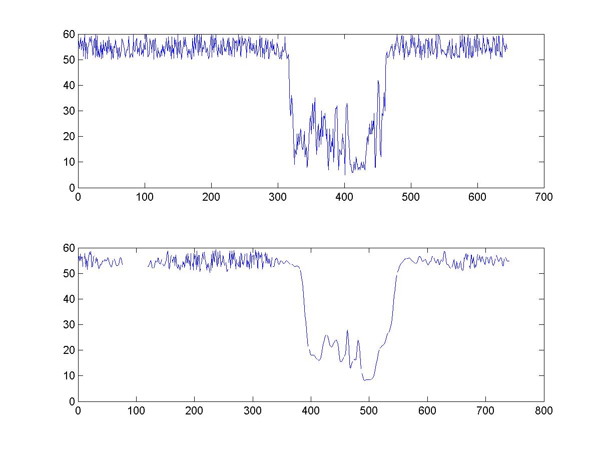
 Implement theKalman Filter (Use identity matrix for statepropagation)or other smoothing filter of your choice on the enclosed “speed24.csv” .Compare the filtered and the original data in a time-series plot (x: timeinterval, y: speed data). Report ME, MAE, and MAPE of the filtering results. Ifthe filter contains any parameters, e.g.smoothing window,smoothing coefficient, experiment to find the best fittingparameters that produces the best trend of the original data.( 平滑窗口，平滑参数，试验找到最好的拟合参数以得到原始数据的最好趋势。)

以下是matlab实现的算法

[plain]  view plain  copy

 

1. function xdense = linear_interp(x, t, tdense)  
2. xdense = zeros(size(tdense));  
3.   
4. for i = 1:length(tdense)  
5.     ind_b = find(tdense(i) >= t, 1, 'last');  
6.     if isempty(ind_b)  
7.         ind_b = 1;  
8.         ind_e = 1;  
9.         lambda = 1;  
10.     elseif ind_b == length(t)  
11.         ind_e = ind_b;  
12.         lambda = 0;  
13.     else  
14.         ind_e = ind_b + 1;  
15.         lambda = (tdense(i) - t(ind_b)) / (t(ind_e) - t(ind_b));  
16.     end;  
17.       
18.     xdense(i) = (1 - lambda) * x(ind_b) + lambda * x(ind_e);  
19. end;  

[plain]  view plain  copy

 

1. %--------------------------------------------------------------------------  
2. % apply fourier analysis on each window size, estimate the dominant  
3. % frequency, and remove high freqs...  
4.   
5. % partition the signals and perform fourier analysis so that we get the  
6. % dominant freq, then smooth the signal using sigma that changes with the  
7. % dominant freq...  
8. %--------------------------------------------------------------------------  
9.   
10. clear all;  
11. %clc;  
12. %close all;  
13.   
14. % 可以调整的参数  
15. windowSize = 41;  
16.   
17. % step 1: read signals from input file  
18. FILE_PATH = 'E:\data.csv';  
19. signal = CSVREAD(FILE_PATH);  
20. S_signal = signal;  
21.   
22.   
23. smoothed_result = zeros(length(signal), 1);  
24.   
25. % 不考虑NAN数据  
26. nan = isnan(signal);  
27. an = ~isnan(signal);  
28. signal = signal(~isnan(signal));  
29.   
30. n = length(signal);  
31. starts = 1:windowSize:n;  
32. if starts(end) + windowSize > n  
33.     starts(end) = n - windowSize + 1;  
34. end;  
35.   
36. dominantSigmas_sample = zeros(length(starts), 1);  
37.   
38. % perform fourier analysis.  
39. for i = 1:length(starts)  
40.     sel = starts(i):starts(i)+windowSize-1;  
41.     coeffs = fft(signal(sel) - mean(signal(sel)));  
42.     % find the dominant one...  
43.     [maxVal, maxIndex] = max(abs(coeffs(1:floor(windowSize/2))));  
44.     dominantSigmas_sample(i) = windowSize / maxIndex/5;  
45. end;  
46.   
47. % simple local linear interpolate...  
48. dominantSigmas = linear_interp(dominantSigmas_sample, starts + windowSize/2, (1:n)');  
49.   
50. smoothed_signal = zeros(n, 1);  
51. % then smooth the signal   
52. for i = 1:n  
53.     % blur the image locally...  
54.     sigma = dominantSigmas(i);  
55.     % 高斯函数分布特性，  
56.     % http://blog.csdn.net/fullyfulei/article/details/8758372  
57.     span = round(3*sigma);  
58.       
59.     sel = (max(1, i - span):min(n, i + span))';  
60.     filter = exp(- (sel - i).^2 / 2 / sigma^2);  
61.       
62.     smoothed_signal(i) = sum(signal(sel) .* filter) / sum(filter);  
63. end  
64. smoothed_result(nan) = NaN;   
65. smoothed_result(an) = smoothed_signal;  
66. maxPoint = [false; smoothed_result(2:end-1) > smoothed_result(3:end) & smoothed_result(2:end-1) > smoothed_result(1:end-2); false];  
67. minPoint = [false; smoothed_result(2:end-1) < smoothed_result(3:end) & smoothed_result(2:end-1) < smoothed_result(1:end-2); false];  
68.   
69. figure  
70. subplot(2,1,1)  
71. plot(S_signal);  
72. subplot(2,1,2)  
73. plot(smoothed_result);  
74.   
75.   
76.   
77. % ME, MAE, MAPE  
78. E = smoothed_signal - signal;  
79. AE = abs(E);  
80.   
81. ME = sum(E)/n;  
82. MAE = sum(AE)/n;  
83. MAPE = sum(abs(E./signal))/n;