经典论文-MobileNetV3论文及实践

2019-MobileNetV3

MobileNetV3: Searching for MobileNetV3

MobileNetV3: 搜索MobileNetV3

• 作者：Andrew Howard, Mark Sandler, Grace Chu, Liang-Chieh Chen, Bo Chen, Mingxing Tan, Weijun Wang, Yukun Zhu, Ruoming Pang, Vijay Vasudevan, Quoc V. Le, Hartwig Adam
• 单位：Google

• 论文地址： https://arxiv.org/abs/1905.02244.pdf
• 项目地址：https://github.com/d-li14/mobilenetv3.pytorch

摘要

我们展示了基于互补搜索技术和新颖架构设计相结合的下一代 MobileNets。MobileNetV3通过结合硬件感知网络架构搜索（NAS）和 NetAdapt算法对移动设计如何协同工作，利用互补的方法来提高移动端CPU推理整体水平。通过这个过程，创建了两个新的发布的 MobileNet模型：MobileNetV3-Large 和 MobileNetV3-Small，分别针对高资源和低资源用例。然后将这些模型应用于目标检测和语义分割。针对语义分割（或任何密集像素预测）任务，提出了一种新的高效分割解码器 Lite reduce Atrous Spatial Pyramid Pooling（LR-ASPP）。实现了移动端分类，检测和分割的最新SOTA成果。与 MobileNetV2 相比，MobileNetV3-Large 在 ImageNet 分类上的准确率提高了 3.2%，同时延迟降低了 20%。与 MobileNetV2 相比，MobileNetV3-Small 的准确率高 6.6%，同时延迟相当。 MobileNetV3-Large 检测速度比 MobileNetV2 快 25%，在COCO检测上的精度大致相等。MobileNetV3-Large LR-ASPP 的速度比 MobileNetV2 R-ASPP 快 30%，在 Cityscapes segmentation分割数据集上，MobileNetV3-Large LR-ASPP 比 MobileNet V2 R-ASPP 快 34%。

1. 简介

高效的神经网络在移动应用程序中变得无处不在，从而实现全新的设备上的体验**。这也是个人隐私的关键推动者，允许用户获得神经网络的好处，而不需要将数据发送到服务器进行评估**。神经网络效率的提升不仅通过更高的精度和更低的延迟来改善用户体验，还通过降低功率损耗来帮助保持电池寿命。

本文描述了开发 MobilenetV3 大型和小型模型的方法，以提供下一代高精度高效的神经网络模型来驱动设备上的计算机视觉。新的网络推动了最新技术的发展，并展示了如何将自动化搜索与新的体系结构进步结合起来，以构建有效的模型。

本文的目标是开发最佳的移动计算机视觉架构，以优化移动设备上的精确延迟交换。为了实现这一点，引入了**(1) 互补搜索技术，(2)适用于移动设备的非线性的新高效版本，(3)新的高效网络设计，(4)一个新的高效分割解码器。**提供了深入的实验，以证明每种技术在广泛的用例和移动电话上评估的有效性和价值。

论文组织如下，从第二节中有关工作的讨论开始，第三节回顾了用于移动模型的高效构建块，第四节回顾了体系结构搜索以及 MnasNet 和 NetAdapt 算法的互补性，第五节描述了通过联合搜索提高模型效率的新型架构设计，第六节介绍了大量的分类，检测和分割实验，以证明有效性和理解不同元素的贡献，第七节载有结论和今后的工作。

2. 相关工作

设计深度神经网络结构来实现精度和效率之间的最优平衡是近年来一个活跃的研究领域，无论是新颖的手工设计结构还是算法神经结构搜索，都在这一领域发挥了重要作用。

SqueezeNet【22】广泛使用带有挤压和扩展模块的1x1 卷积，主要集中于减少参数的数量。最近的工作将关注点从减少参数转移到减少操作的数量（MAdds）和实际测量的延迟。MobileNetV1【19】采用深度可分离卷积，大大提高了计算效率。MobileNetV2【39】在此基础上进行了扩展，引入了一个具有反向残差和线性瓶颈的资源高效块。ShuffleNet【49】利用组卷积和信道洗牌操作进一步减少 MAdds。CondenseNet【21】在训练阶段学习组卷积，以保持层与层之间有用的紧密连接，以便特征重用。ShiftNet【46】提出了与点向卷积交织的移位操作，以取代昂贵的空间卷积。

为了使体系结构设计过程自动化，首先引入了强化学习（RL）来搜索具有竞争力的精度的高效体系结构【53， 54， 3， 27， 35】。一个完全可配置的搜索空间可能会以指数级增长且难以处理。因此，早期的架构搜索工作主要关注单元级结构搜索，并且在所有层中重用相同的单元。最近，【43】探索了一个块级分层搜索空间，允许在网络的不同分辨率块上使用不同的层结构。为了降低搜索的计算成本，在【28， 5， 45】中使用了可微架构搜索框架，并进行了基于梯度的优化。针对现有网络适应受限移动平台的问题，【48， 15， 12】提出了更高效的自动化网络简化算法。

量化【23， 25， 37， 41， 51， 52， 37】是通过降低精度算法来提高网络效率的另一项重要的补充工作。最后，知识蒸馏【4， 17】提供了一种附加的补充方法，在大型“教师”网络的指导下生成精确的小型“学生”网络。

将上述翻译总结一下，即目前常用的一些减少网络计算量的方法：

• 基于轻量化网络设计：比如 MobileNet 系列，ShuffleNet系列，Xception等，使用Group卷积，1*1 卷积等技术减少网络计算量的同时，尽可能的保证网络的精度。
• 模型剪枝：大网络往往存在一定的冗余，通过减去冗余部分，减少网络计算量。
• 量化：利用 TensorRT 量化，一般在 GPU 上可以提速几倍
• 知识蒸馏：利用大模型（teacher model）来帮助小模型（student model）学习，提高 student modelde 精度。

MobileNet系列当然是典型的第一种方法。

3. 高效的移动构建块

移动模型已经建立在越来越高效的构建块上。MobileNetV1【17】引入深度可分离卷积作为传统卷积层的有效替代。深度可分离卷积通过将空间滤波与特征生成机制分离，有效的分解了传统卷积。深度可分离卷积由两个独立的层定义：用于空间滤波的轻量级深度卷积和用于特征生成的较重的1*1点卷积。

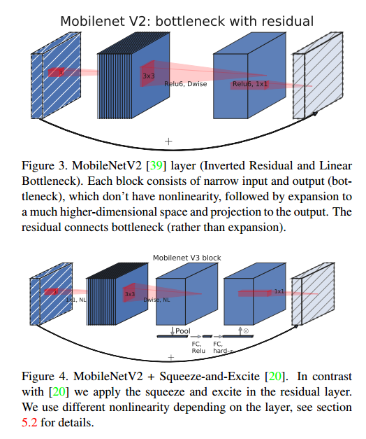
MobileNetV2【37】引入了线性瓶颈和反向残差结构，以便利用问题的低秩性质使层结构更加有效。这个结构如图3所示，由1*1 展开卷积，深度卷积和1*1 投影层定义。当且仅当它们具有相同数量的通道时，输入和输出才通过剩余连接进行连接。这种结构在输入和输出处保持了紧凑的表示，同时在内部扩展到高维特征空间，以便增加非线性每个通道转换的表达能力。

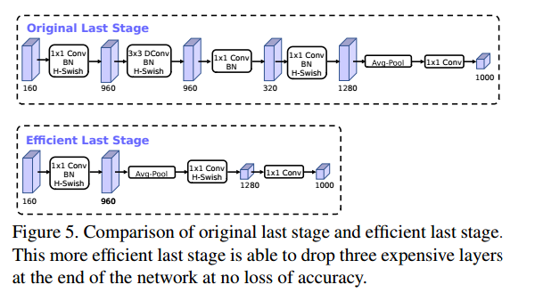
MnasNet 建立在 MobileNetV2 结构上，通过在瓶颈结构中引入基于挤压和激励的轻量级注意模块。注意：与【20】中提出的基于 ResNet 的模块相比，挤压和激励模块集成在不同的位置。模块位于展开中的深度过滤器之后，以便注意应用于最大的表示，如图4所示。

对于MobileNet V3，使用这些层的组合作为构建块，以便构建最有效的模型。层也升级修改成 swish 非线性【34】。挤压和激励以及 swish 非线性都使用了 Sigmoid，它的计算效率很低，而且很难在定点算法中保持精度，因此将其替换为hard Sigmoid，如5.2 节所讨论的。

4. 网络搜索

网络搜索已被证明是发现和优化网络架构的一个非常强大的工具【53，43，5，48】。对于MobilenetV3，使用平台感知的 NAS 通过优化每个网络块来搜索全局网络结构。然后，使用 NetAdapt 算法搜索每个层的过滤器数量。这些技术是互补的，可以结合起来为给定的硬件平台有效的找到优化模型。

4.1 使用NAS感知平台进行逐块（Block-wise）搜索

与【43】类似，我们采用平台感知神经结构方法来寻找全局网络结构。由于使用相同的基于RNN的控制器和相同的分解层次搜索空间，所以对目标延迟在 80ms 左右的大型移动模型，找到了与【43】类似的结果。因此，我们只需重用相同的MnasNet-A1 [43]作为最初的大型移动模型，然后在其之上应用NetAdapt [48]和其他优化。

然而，发现原始的奖励设计并没有针对小型手机模型进行优化。具体来说，它使用一个多目标奖励 $ACC(m)\ast [LAT(m)/TAR{]}^w$ 来近似 pareto 最优解，根据目标延迟 TAR 为每个模型 m 平衡模型精度 ACC(m) 和延迟 LAT(m) ，可以观察到精度变化更显著延迟小模型，因此，需要一个较小的权重系数 w=-0.15（vs 原始 w=-0.07）来弥补大精度变化不同的延迟。在新的权重因子 w 的增强下，从头开始一个新的架构搜索，以找到初始的 seed 模型，然后应用 NetAdapt 和其他优化来获得最终的 MobileNetV3-Small模型。

4.2 使用NetAdapt 进行 Layerwise 搜索

在架构搜索中使用的第二种技术是 NetAdapt【48】。这种方法是对平台感知 NAS 的补充：它允许以顺序的方式对单个层进行微调，而不是试图推断出粗糙但全局的体系结构。详细请参阅原文。简而言之，这项技术的进展如下：

• 1 从平台感知 NAS 发现的种子网络体系结构开始
• 2 对于每一个步骤：
  • 提出一套新的提议proposal， 每个提议都表示对体系结构的修改，与前一步相比，该体系结构至少可以减少延迟
  • 对于每一个提议，使用前一个步骤的预先训练的模型，并填充新提出的架构，适当地截断和随机初始化缺失的权重。对于 T 步的每个建议进行微调，以获得对精度的粗略估计
  • 根据某种标准选择最佳提议proposal
• 3 重复前面的步骤，直到达到目标延迟。

在【48】中，度量标准是为了最小化精度的变化。我们修改了这个算法，使延迟变化和精度变化的比例最小化。也就是说，对于每个 NetAdapt 步骤中生成的所有建议，选择一个最大化的建议： ACC/latency 。延迟满足2(a)中的约束。直觉告诉我们，由于建议是离散的，所以更喜欢最大化权衡曲线斜率的建议。

这个过程重复进行，直到延迟达到目标，然后从头开始重新培训新的体系结构。使用与在【46】中为 MobileNetV2 相同的建议proposal生成器。 具体来说，允许以下两种建议：

• 减少任何扩展层的尺寸
• 减少共享相同瓶颈大小的所有块中的瓶颈——以维护残差连接

在实验中，使用 T=10000，并发现虽然它增加了提案的初始微调的准确性。然而，当从头开始训练时，它通常不会改变最终的精度。设 $\delta =0.01|L|$，其中L为种子模型的延迟。

5. 网络提升

除了网络搜索，还为模型引入了一些新的组件，以进一步改进最终模型。在网络的开始和结束阶段，重新设计了计算昂贵的层。还引入了一种新的非线性，h-swish，它是最近的 swish非线性的改进版本，计算速度更快，更易于量化。

5.1 重新设计昂贵的层

一旦通过架构搜索找到seed模型后就会发现，一些最后的层以及一些较早的层比其他层更昂贵。建议对体系结构进行一些修改，以减少这些慢层的延迟，同时保持准确性，这些修改超出了当前搜索空间的范围。

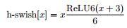
第一个修改将重新处理网络的最后几层是如何交互的，以便生成最终层功能更有效率。目前的模型基于 MobileNetV2 的倒瓶颈结构和使用 1*1 卷积变体作为最后一层，以扩展高维特征空间。这一层非常重要，因为它具有丰富的预测特征。然而，这是以额外的延迟为代价的。

为了减少延迟并保留高维特征，可以将该层移到最终的平均池之外。最后一组特征现在计算为 1*1 空间分辨率，而不是 7*7 的空间分辨率。这种设计选择的结果是，在计算和延迟方面，特征的计算变得几乎是免费的。

一旦降低了该特征生成层的成本，就不再需要以前的瓶颈投影层来减少计算量。 该观察允许我们删除前一个瓶颈层中的投影和过滤层，从而进一步降低计算复杂度。原始阶段和优化后的阶段如图5所示，有效的最后一个阶段将延迟减少 10毫秒，即 15% 的运行时间，并将操作数量减少了 3000 万个 MAdd ，几乎没有损失精度。第六节包含了详细的结果。

另一个昂贵的层是初始化卷积器集。目前的移动模型倾向于在一个完整的 3*3 卷积中使用 32个滤波器来构建初始滤波器库进行边缘检测。通常这些过滤器是彼此的镜像，我们尝试减少滤波器的数量，并使用不同的非线性来尝试减少冗余。决定对这一层使用硬 swish 非线性，并和其他非线性函数进行对比测试，将过滤器的数量减少到 16 个，同时保持与使用 ReLU 或 swish 的 32个过滤器相同的精度，这节省了额外的 3 毫秒和 1000 万次 MAdds。

5.2 非线性

在【36,13,16】中引入了一种称为 swish 的非线性，当作为 ReLU 的替代时，它可以显著提高神经网络的精度。非线性定义为：

虽然这种非线性提高了精度，但是在嵌入式环境中，它的成本是非零的，因为在移动设备上计算Sigmoid函数要昂贵的多。用两种方法处理这个问题。

• 将 Sigmoid 函数替换为它的分段线性硬模拟：ReLU6(x + 3)/6，类似于【11, 44】。较小的区别是，使用的是 ReLU6，而不是自定义的裁剪常量。类似的，Swish的硬版本h-swish也变成了

​ 最近在【2】中也提出了类似的 hard-swish 版本。图6显示了 Sigmoid和 Swish 非线性的软，硬版本的比较。选择常量的动机是简单，并且与原始的平滑版本很好地匹配。在实验中，发现所有这些函数的硬版本在精度上没有明显的差异，但是从部署的角度来看，它们具有多种优势。首先，几乎所有的软件和硬件框架上都可以使用 ReLU6 的优化实现。其次，在量化模式下，它消除了由于近似 Sigmoid 的不同实现而带来的潜在的数值精度损失。最后，即使优化了量化的 Sigmoid实现，其速度也比相应的 ReLU 慢的多。在实验中，使用量化模式下的 swish 替换 h-swish 使推理延迟增加了 15%。

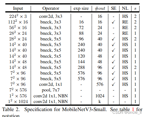
• 随着深入网络，应用非线性的成本会降低，因为每层激活内存通常在分辨率下降时减半。另外发现 swish 的大多数好处都是通过只在更深的层中使用它们实现的。因此，在架构中，只在模型的后半部分使用 h-swish。参照表1和表2来获得精确的布局。

即使有了这些优化，h-swish仍然会引入一些延迟成本。然而，正如第6节中所演示的，当使用基于分段函数的优化实现时，在没有进行优化的前提下对精度和延迟的净影响是正向的，而且是实质性的。

5.3 大的压缩和激活

在【43】中，压缩和激活瓶颈的大小与卷积瓶颈的大小有关。取而代之的是，这里将它们全部替换为固定为膨胀层通道数的 1/4。发现这样做可以在适当增加参数数量的情况下提高精度，并没有明显的延迟成本。

5.4 MobileNetV3 定义

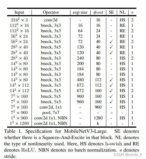
MobileNetV3 被定义为两个模型：MobileNetV3-Large 和 MobileNetV3-Small。这些模型针对的是高资源用例和低资源用例。通过应用平台感知的 NAS 和 NetAdapt 进行网络搜索，并结合本节定义的网络改进，可以创建模型，网络的完整结构见表1和表2。

6. 实验

做了各种实验来证明新的 MobileNet V3模型的有效性。总结分析在分类，检测和分割任务上的实验结果。另外也进行了各种消融研究，以阐明各种设计决策对模型性能的影响。

6.1 分类

由于ImageNet数据集已经成为一种标准，我们在所有分类实验中都是在 ImageNet【38】上进行的，并将准确度与各种资源实验度量方法（如延迟和乘法加法（MAdds））进行比较。

6.1.1 训练设置

在 4*4 TPU Pod【24】上使用 0.9 动量的标准 TensorFlow RMSProp Optimizer 进行同步训练。初始学习率设置为 0.1， 批次大小为 4096（每个芯片 128 张图片），学习率衰减率为 0.01 每三个epoch， dropout设置为 0.8 ，l2 的权重衰减为 1e-5，预处理操作和 Inception【40】相同。最后，使用衰减为 0.9999 的指数滑动平均。所有的卷积层都使用批次处理归一化层，平均衰减为 0.99。

6.1.2 测试设置

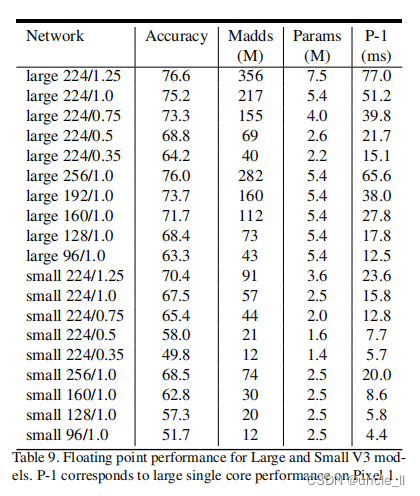
为了测试延迟，使用标准的谷歌像素手机，并通过标准的 TFLite 基准测试工具运行所有网络。在所有测试中都使用单线程大内核。这里没有报告多核推理时间，因为我们发现这种设置对移动应用程序不太实用。我们为TFLite提供了一个h-swish操作符，现在在TFLite最新版本中是默认的。在图9中展示了优化后的h-swish的影响。

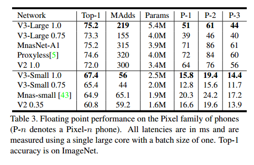
上图为作者在ImageNet网络的测试结果，结果可以看出 V3 Large 相比较于 V2 1.0 精度上提高了大约3个点，但是速度上从 64降到了51（Pixel-1 手机），V3 small 相较于 V2 0.35 ，精度提升了大约 7个点，速度稍有提升，从 16.5ms 到 15.8ms（Pixel-1 手机）

6.2 结果

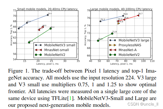
图1，Pixel 1 延迟与 top-1 ImageNet 准确性之间的权衡。输入大小都是224，大V3和小V3使用乘数 0.75,1和1.25显示最佳边界。所有延迟都是使用 TFLite【1】在同一设备的单个大内核上测量的。MobileNetV3-Small和 Large是建议的下一代移动模型。

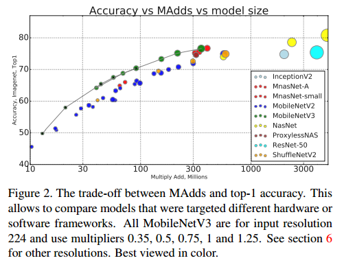
图2：MAdds 和 top-1 精度之间的衡量。这允许比较针对不同硬件或软件框架的模型。所有 MobileNet V3 的输入分辨率均为 224，并使用乘数 0.35， 0.5， 0.75， 1 和 1.25。

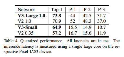
如图1所示，MV3模型优于目前的技术状态，如 MnasNet，ProxylessNas 和 MobileNetV2。在表3中报告了不同像素手机上的浮点性能，在表4中展示了量化的结果。模型量化后（float量化，非int8量化）的耗时，其中P-1，P-2，P-3 分别代表的是不同性能的手机。相较于MobileNetV2， V3-Large网络的Top-1 精度从70.9 上升到 73.8ms，在P1-P3的加速效果来看P1 加速了 8ms，P2加速了6ms，P-3加速了5ms，与V2网络相比，提速快一些，但V3-Small 在量化后提速效果相较于V2并不明显。

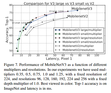
在图7中，展示了MobileNet V3 性能权衡作为乘法和分辨率的函数。注意到，MobileNetV3-Small 的性能比 MobilenetV3-Large 的性能好很多，其乘法器缩放到与性能匹配的倍数接近3%。另一方面，分辨率提供了一个比乘数更好的权衡。但需要注意的是，分辨率通常是由问题决定的（例如分割和检测问题通常需要更高的分辨率），因此不能总是用作可调参数。 实验了使用不同分辨率以及不同的模型深度的精度的对比，分辨率分别选择的是【96,128,160,192,224,256】，深度分辨选为原来的【0.35,0.5,0.75,1.0,1.25】。可见，其实resolution 对于精度以及速度的平衡效果更好，可以达到更快的速度，同时精度没有改变模型深度低，反而更高。

6.2.1 　消融实验

非线性的影响 研究在哪里插入非线性 h-swish 以及使用优化实现比使用朴素实现的改进。从表5可看出，使用一个优化的 h-swish 节省 6 ms（超过 10%的运行时长）。优化后的h-swish 比起 传统的 ReLU 只会增加一个额外 1ms

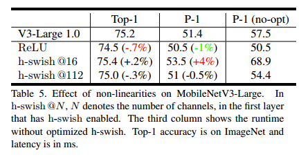
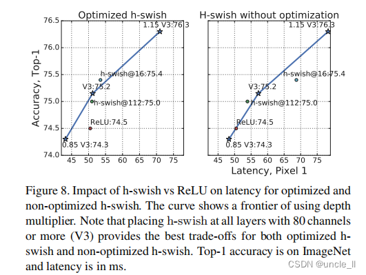
图8显示了基于非线性的选择和网络的有效边界宽度。MobileNetV3 使用 h-swish 中间的网络和支配 ReLU。有趣的是要注意，添加 h-swish 整个网络是略优于插值扩大网络的前沿。

其他组件的影响 在图9中，展示了不同组件的引入是如何沿着延迟/准确率曲线移动的。

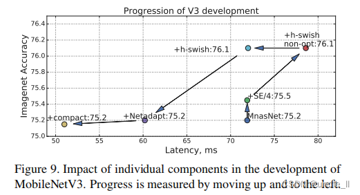
上图展示了MobileNet V3中单个组件的影响，过程是测试移动到右边。

6.3 检测

使用 MobileNet V3作为SSDLite的骨干特征提取器的替代，并与COCO dataset上与其他骨干网络进行了对比。

在MobileNet V2之后，将第一层 SSDLite 附加到输出步长为 16 的最后一个特征提取器层，并将第二层 SSDLite 附加到输出步长为 32 的最后一个特征提取器层。根据检测文献，将这两个特征提取层分别称为 C4和 C5。对于MobileNet V3-Large，C4是第13 个瓶颈块的膨胀层。对于 MobileNetV3-Small ，C4是第9个瓶颈层的膨胀层。但对这两个网络，C5都是池化层之前的一层。

此外还将 C4和 C5之间的所有特征层的通道数减少2倍。这是因为 MobileNetV3的最后几层被调优为输出 1000 类，当将 90 个类转移到 COCO 时，这可能是多余的。

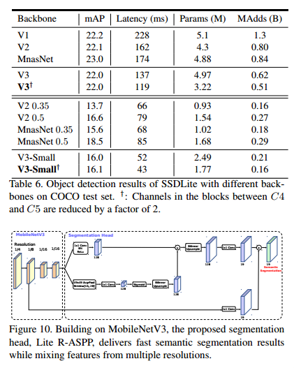
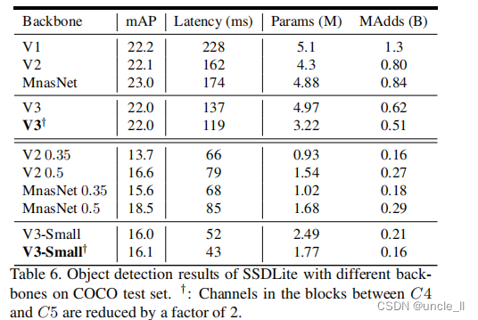
COCO 测试集的结果如表6所示。在通道缩减的情况下，MobileNetV3-Large 比具有几乎相同精度mAP的 MobileNetV2快 25%。在相同的延迟下，MobileNet V3 比 MobileNet V2和 MnasNet 高 2.4 和 0.5 。对于这两种 MobileNet V3模型，通道减少技巧在没有丢失mAP的情况下可以减少大约 15% 的延迟，这表明 ImageNet 分类和 COCO对象检测可能更喜欢不同的特征提取器形状。

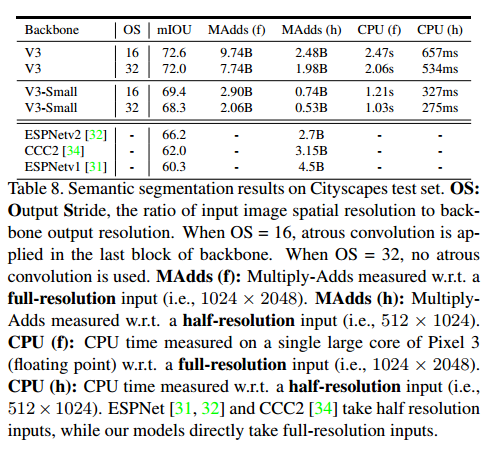
6.4 语义分割

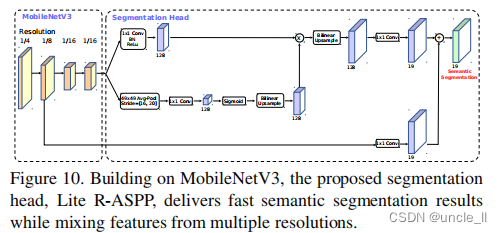
在本小节中，使用 MobileNetV2 和提出的 MobileNetV3作为移动语义分割的网络骨架。此外，比较了两个分割头。第一个是在 【39】中提出的 R-ASPP。R-ASPP是一种无源空间金字塔池化模块的简化设计，它是采用由1x1个卷积和一个全局平均池化操作组成的两个分支。在本文中，提出了另一种轻量级分割头，称为 Lite R-ASPP（或 LR-ASPP），如图10所示，Lite R-ASPP是对 R-ASPP的改进，它部署全局平均池化的方式类似于挤压-激活模块，其中使用了一个大的池化核，具有较大的步长（以节省一些计算），并且模块中只有 一个1x1 个卷积。并对 MobileNet V3 的最后一个块应用 Atrous Conv 来提取更密集的特征，并进一步从底层特性添加一个skip连接来捕获更详细的信息。

使用CityScapes 数据集进行实验，只使用了其中一些fine 标注数据，并使用mIOU评价指标。采用与【8,3 9】相同的训练方案, 所有的模型都是从零开始训练，没有使用ImageNet[36] 进行预训练，并且使用单尺度输入进行评估。与目标检测类似，发现可以在不显著降低性能的情况下，将网络主干最后一块的通道减少2倍。我们认为这是因为主干网络设计了 1000 类 ImageNet 图像分类，而Cityscapes 只有 19类，这意味着主干网络存在一定的通道冗余。

在表7中报告了我们的城市景观验证集的结果。 7.如表中所示，我们观察到(1)减少最后一块网络骨干的通道2倍显著提高了速度同时保持类似的性能（第1行和第2行，行5行6），(2)提出分割头LR-ASPP略快于R-ASPP [39]而性能提高（行2行3，行6行7），(3)减少过滤器分割头从256年到128年提高速度的性能稍差(第3行对第4行，第7行。(4)当使用相同的设置时，MobileNetV3模型变体获得了类似的性能，同时比MobileNetV2略快(第1行vs第5行，第2行vs第6行，第3行与第7行，第4行vs。第8行)，(5)移动eNetV3-Small的性能与移动eNetV2-0.5相似，但速度更快；(6)移动eNetV3-Small明显优于MobileNetV2-0.35，同时产生相似的速度。

7. 总结和未来工作

在这篇文章中，我们介绍了 MobilenetV3大大小小的模型，展示了在移动分类，检测和分割方面的最新技术。我们利用多种类型的网络架构搜索以及先进的网络设计，以交付下一代移动模型。此外还展示了如何适应非线性，如swish 和应用压缩和激励的量化友好和有效的方式，将它们作为有效的工具引入移动模型领域。还介绍了一种新的轻量级分割解码器，称为 LR-ASPP。尽管如何将自动搜索技术与人类直觉最好地结合起来仍然是一个悬而未决的问题，但我们很高兴的展示了这些初步的积极结果，并将在未来的工作中继续改进这些方法。

参考文献

• [1] Mart´ın Abadi, Ashish Agarwal, Paul Barham, Eugene Brevdo, Zhifeng Chen, Craig Citro, Greg S. Corrado, Andy Davis, Jeffrey Dean, Matthieu Devin, Sanjay Ghemawat, Ian Goodfellow, Andrew Harp, Geoffrey Irving, Michael Isard, Yangqing Jia, Rafal Jozefowicz, Lukasz Kaiser, Manjunath Kudlur, Josh Levenberg, Dan Man´e, Rajat Monga, Sherry Moore, Derek Murray, Chris Olah, Mike Schuster, Jonathon Shlens, Benoit Steiner, Ilya Sutskever, Kunal Talwar, Paul Tucker, Vincent Vanhoucke, Vijay Vasudevan, Fernanda Vi´egas, Oriol Vinyals, Pete Warden, Martin Wattenberg, Martin Wicke, Yuan Yu, and Xiaoqiang Zheng. TensorFlow: Large-scale machine learning on heterogeneous systems, 2015. Software available from tensorflflow.org.
• [2] R. Avenash and P. Vishawanth. Semantic segmentation of satellite images using a modifified cnn with hard-swish activation function. In VISIGRAPP, 2019. 2, 4
• [3] Bowen Baker, Otkrist Gupta, Nikhil Naik, and Ramesh Raskar. Designing neural network architectures using reinforcement learning. CoRR, abs/1611.02167, 2016. 2
• [4] Cristian Bucilua, Rich Caruana, and Alexandru NiculescuMizil. Model compression. In Proceedings of the 12th ACM SIGKDD International Conference on Knowledge Discovery and Data Mining, KDD ’06, pages 535–541, New York, NY, USA, 2006. ACM. 2
• [5] Han Cai, Ligeng Zhu, and Song Han. Proxylessnas: Direct neural architecture search on target task and hardware. CoRR, abs/1812.00332, 2018. 2, 3, 6
• [6] Liang-Chieh Chen, George Papandreou, Iasonas Kokkinos, Kevin Murphy, and Alan L Yuille. Semantic image segmentation with deep convolutional nets and fully connected crfs. In ICLR, 2015. 7
• [7] Liang-Chieh Chen, George Papandreou, Iasonas Kokkinos, Kevin Murphy, and Alan L Yuille. Deeplab: Semantic image segmentation with deep convolutional nets, atrous convolution, and fully connected crfs. TPAMI, 2017. 7
• [8] Liang-Chieh Chen, George Papandreou, Florian Schroff, and Hartwig Adam. Rethinking atrous convolution for semantic image segmentation. CoRR, abs/1706.05587, 2017. 7, 8
• [9] Liang-Chieh Chen, Yukun Zhu, George Papandreou, Florian Schroff, and Hartwig Adam. Encoder-decoder with atrous separable convolution for semantic image segmentation. In ECCV, 2018. 7
• [10] Marius Cordts, Mohamed Omran, Sebastian Ramos, Timo Rehfeld, Markus Enzweiler, Rodrigo Benenson, Uwe Franke, Stefan Roth, and Bernt Schiele. The cityscapes dataset for semantic urban scene understanding. In CVPR, 2016. 7
• [11] Matthieu Courbariaux, Yoshua Bengio, and Jean-Pierre David. Binaryconnect: Training deep neural networks with binary weights during propagations. CoRR, abs/1511.00363, 2015. 2, 4
• [12] Xiaoliang Dai, Peizhao Zhang, Bichen Wu, Hongxu Yin, Fei Sun, Yanghan Wang, Marat Dukhan, Yunqing Hu, Yiming Wu, Yangqing Jia, Peter Vajda, Matt Uyttendaele, and Niraj K. Jha. Chamnet: Towards effificient network design through platform-aware model adaptation. CoRR, abs/1812.08934, 2018. 2
• [13] Stefan Elfwing, Eiji Uchibe, and Kenji Doya. Sigmoid weighted linear units for neural network function approximation in reinforcement learning. CoRR, abs/1702.03118, \2017. 2, 4
• [14] Mark Everingham, S. M. Ali Eslami, Luc Van Gool, Christopher K. I. Williams, John Winn, and Andrew Zisserma. The pascal visual object classes challenge a retrospective. IJCV, 2014. 7
• [15] Yihui He and Song Han. AMC: automated deep compression and acceleration with reinforcement learning. In ECCV, 2018. 2
• [16] Dan Hendrycks and Kevin Gimpel. Bridging nonlinearities and stochastic regularizers with gaussian error linear units. CoRR, abs/1606.08415, 2016. 2, 4
• [17] Geoffrey Hinton, Oriol Vinyals, and Jeffrey Dean. Distilling the knowledge in a neural network. In NIPS Deep Learning and Representation Learning Workshop, 2015. 2
• [18] Matthias Holschneider, Richard Kronland-Martinet, Jean Morlet, and Ph Tchamitchian. A real-time algorithm for signal analysis with the help of the wavelet transform. In Wavelets: Time-Frequency Methods and Phase Space, pages 289–297. Springer Berlin Heidelberg, 1989. 7
• [19] Andrew G. Howard, Menglong Zhu, Bo Chen, Dmitry Kalenichenko, Weijun Wang, Tobias Weyand, Marco Andreetto, and Hartwig Adam. Mobilenets: Effificient convolutional neural networks for mobile vision applications. CoRR, abs/1704.04861, 2017. 2
• [20] J. Hu, L. Shen, and G. Sun. Squeeze-and-Excitation Networks. ArXiv e-prints, Sept. 2017. 2, 3, 7
• [21] Gao Huang, Shichen Liu, Laurens van der Maaten, and Kilian Q. Weinberger. Condensenet: An effificient densenet using learned group convolutions. CoRR, abs/1711.09224, 2017. 2
• [22] Forrest N. Iandola, Matthew W. Moskewicz, Khalid Ashraf, Song Han, William J. Dally, and Kurt Keutzer. Squeezenet: Alexnet-level accuracy with 50x fewer parameters and <1mb model size. CoRR, abs/1602.07360, 2016. 2
• [23] Benoit Jacob, Skirmantas Kligys, Bo Chen, Menglong Zhu, Matthew Tang, Andrew Howard, Hartwig Adam, and Dmitry Kalenichenko. Quantization and training of neural networks for effificient integer-arithmetic-only inference. In The IEEE Conference on Computer Vision and Pattern Recognition (CVPR), June 2018. 2
• [24] Norman P. Jouppi, Cliff Young, Nishant Patil, David A. Patterson, Gaurav Agrawal, Raminder Bajwa, Sarah Bates, Suresh Bhatia, Nan Boden, Al Borchers, Rick Boyle, Pierreluc Cantin, Clifford Chao, Chris Clark, Jeremy Coriell, Mike Daley, Matt Dau, Jeffrey Dean, Ben Gelb, Tara Vazir Ghaemmaghami,Rajendra Gottipati, William Gulland, Robert Hagmann, Richard C. Ho, Doug Hogberg, John Hu, Robert Hundt, Dan Hurt, Julian Ibarz, Aaron Jaffey, Alek Jaworski, Alexander Kaplan, Harshit Khaitan, Andy Koch, Naveen Kumar, Steve Lacy, James Laudon, James Law, Diemthu Le, Chris Leary, Zhuyuan Liu, Kyle Lucke, Alan Lundin, Gordon MacKean, Adriana Maggiore, Maire Mahony, Kieran Miller, Rahul Nagarajan, Ravi Narayanaswami, Ray Ni, Kathy Nix, Thomas Norrie, Mark Omernick, Narayana Penukonda, Andy Phelps, Jonathan Ross, Amir Salek, Emad Samadiani, Chris Severn, Gregory Sizikov, Matthew Snelham, Jed Souter, Dan Steinberg, Andy Swing, Mercedes Tan, Gregory Thorson, Bo Tian, Horia Toma, Erick Tuttle, Vijay Vasudevan, Richard Walter, Walter Wang, Eric Wilcox, and Doe Hyun Yoon. In-datacenter performance analysis of a tensor processing unit. CoRR, abs/1704.04760, 2017. 5
• [25] Raghuraman Krishnamoorthi. Quantizing deep convolutional networks for effificient inference: A whitepaper. CoRR, abs/1806.08342, 2018. 2
• [26] Tsung-Yi Lin, Michael Maire, Serge Belongie, James Hays, Pietro Perona, Deva Ramanan, Piotr Doll´ar, and C Lawrence Zitnick. Microsoft COCO: Common objects in context. In ECCV, 2014. 7
• [27] Chenxi Liu, Barret Zoph, Jonathon Shlens, Wei Hua, Li-Jia Li, Li Fei-Fei, Alan L. Yuille, Jonathan Huang, and Kevin Murphy. Progressive neural architecture search. CoRR, abs/1712.00559, 2017. 2
• [28] Hanxiao Liu, Karen Simonyan, and Yiming Yang. DARTS: differentiable architecture search. CoRR, abs/1806.09055, 2018. 2
• [29] Wei Liu, Andrew Rabinovich, and Alexander C. Berg. Parsenet: Looking wider to see better. CoRR, abs/1506.04579, 2015. 7
• [30] Jonathan Long, Evan Shelhamer, and Trevor Darrell. Fully convolutional networks for semantic segmentation. In CVPR, 2015. 7
• [31] Sachin Mehta, Mohammad Rastegari, Anat Caspi, Linda G. Shapiro, and Hannaneh Hajishirzi. Espnet: Effificient spatial pyramid of dilated convolutions for semantic segmentation. In Computer Vision - ECCV 2018 - 15th European Conference, Munich, Germany, September 8-14, 2018, Proceedings, Part X, pages 561–580, 2018. 8
• [32] Sachin Mehta, Mohammad Rastegari, Linda G. Shapiro, and Hannaneh Hajishirzi. Espnetv2: A light-weight, power effificient, and general purpose convolutional neural network. CoRR, abs/1811.11431, 2018. 8
• [33] George Papandreou, Iasonas Kokkinos, and Pierre-Andre Savalle. Modeling local and global deformations in deep learning: Epitomic convolution, multiple instance learning, and sliding window detection. In CVPR, 2015. 7
• [34] Hyojin Park, Youngjoon Yoo, Geonseok Seo, Dongyoon Han, Sangdoo Yun, and Nojun Kwak. Concentrated comprehensive convolutions for lightweight semantic segmentation. CoRR, abs/1812.04920, 2018. 8
• [35] Hieu Pham, Melody Y. Guan, Barret Zoph, Quoc V. Le, and Jeff Dean. Effificient neural architecture search via parameter sharing. CoRR, abs/1802.03268, 2018. 2
• [36] Prajit Ramachandran, Barret Zoph, and Quoc V. Le. Searching for activation functions. CoRR, abs/1710.05941, 2017. 2, 4
• [37] Mohammad Rastegari, Vicente Ordonez, Joseph Redmon, and Ali Farhadi. Xnor-net: Imagenet classifification using binary convolutional neural networks. CoRR, abs/1603.05279, \2016. 2
• [38] Olga Russakovsky, Jia Deng, Hao Su, Jonathan Krause, Sanjeev Satheesh, Sean Ma, Zhiheng Huang, Andrej Karpathy,Aditya Khosla, Michael Bernstein, Alexander C. Berg, and Li Fei-Fei. Imagenet large scale visual recognition challenge. Int. J. Comput. Vision, 115(3):211–252, Dec. 2015. 5, 8
• [39] Mark Sandler, Andrew G. Howard, Menglong Zhu, Andrey Zhmoginov, and Liang-Chieh Chen. Mobilenetv2: Inverted residuals and linear bottlenecks. mobile networks for classifification, detection and segmentation. CoRR, abs/1801.04381, \2018. 2, 3, 6, 7, 8
• [40] Pierre Sermanet, David Eigen, Xiang Zhang, Micha¨el Mathieu, Rob Fergus, and Yann LeCun. Overfeat: Integrated recognition, localization and detection using convolutional networks. arXiv:1312.6229, 2013. 7
• [41] Daniel Soudry, Itay Hubara, and Ron Meir. Expectation backpropagation: Parameter-free training of multilayer neural networks with continuous or discrete weights. In Zoubin Ghahramani, Max Welling, Corinna Cortes, Neil D. Lawrence, and Kilian Q. Weinberger, editors, NIPS, pages 963–971, 2014. 2
• [42] Christian Szegedy, Sergey Ioffe, and Vincent Vanhoucke. Inception-v4, inception-resnet and the impact of residual connections on learning. CoRR, abs/1602.07261, 2016. 5
• [43] Mingxing Tan, Bo Chen, Ruoming Pang, Vijay Vasudevan, and Quoc V. Le. Mnasnet: Platform-aware neural architecture search for mobile. CoRR, abs/1807.11626, 2018. 2, 3, 5, 6
• [44] SPSE the Society for Imaging Science, Technology, Society of Photo-optical Instrumentation Engineers, and Technical Association of the Graphic Arts. Curves and Surfaces in Computer Vision and Graphics. Number v. 1610 in Proceedings of SPIE–the International Society for Optical Engineering. SPIE, 1992. 4
• [45] Bichen Wu, Xiaoliang Dai, Peizhao Zhang, Yanghan Wang, Fei Sun, Yiming Wu, Yuandong Tian, Peter Vajda, Yangqing Jia, and Kurt Keutzer. Fbnet: Hardware-aware effificient convnet design via differentiable neural architecture search. CoRR, abs/1812.03443, 2018. 2
• [46] Bichen Wu, Alvin Wan, Xiangyu Yue, Peter H. Jin, Sicheng Zhao, Noah Golmant, Amir Gholaminejad, Joseph Gonzalez, and Kurt Keutzer. Shift: A zero flflop, zero parameter alternative to spatial convolutions. CoRR, abs/1711.08141, \2017. 2
• [47] Jiaxiang Wu, Cong Leng, Yuhang Wang, Qinghao Hu, and Jian Cheng. Quantized convolutional neural networks for mobile devices. CoRR, abs/1512.06473, 2015. 2
• [48] Tien-Ju Yang, Andrew G. Howard, Bo Chen, Xiao Zhang, Alec Go, Mark Sandler, Vivienne Sze, and Hartwig Adam. Netadapt: Platform-aware neural network adaptation for mobile applications. In ECCV, 2018. 2, 3
• [49] Xiangyu Zhang, Xinyu Zhou, Mengxiao Lin, and Jian Sun. Shufflflenet: An extremely effificient convolutional neural network for mobile devices. CoRR, abs/1707.01083, 2017. 2
• [50] Hengshuang Zhao, Jianping Shi, Xiaojuan Qi, Xiaogang Wang, and Jiaya Jia. Pyramid scene parsing network. In CVPR, 2017. 7
• [51] Aojun Zhou, Anbang Yao, Yiwen Guo, Lin Xu, and Yurong Chen. Incremental network quantization: Towards lossless cnns with low-precision weights. CoRR, abs/1702.03044, \2017. 2
• [52] Shuchang Zhou, Zekun Ni, Xinyu Zhou, He Wen, Yuxin Wu, and Yuheng Zou. Dorefa-net: Training low bitwidth convolutional neural networks with low bitwidth gradients. CoRR, abs/1606.06160, 2016. 2
• [53] Barret Zoph and Quoc V. Le. Neural architecture search with reinforcement learning. CoRR, abs/1611.01578, 2016. 2, 3
• [54] Barret Zoph, Vijay Vasudevan, Jonathon Shlens, and Quoc V. Le. Learning transferable architectures for scalable image recognition. CoRR, abs/1707.07012, 2017. 2

实现

基于torch1.8版本实现

import os
import sys
import numpy as np
import pandas as pd
from matplotlib import pyplot as plt
from typing import Any

import torch
import torch.nn as nn
import torch.nn.init as init
import torch.nn.functional as f
import torch.optim as optim
from torch.utils.data import Dataset, DataLoader
import torchvision

# 设置运行环境
os.environ['CUDA_VISIABLE_DIVICES'] = '0, 1'

# 设置超参数
batch_size = 64
lr = 1e-4
num_works = 8
epochs = 100


from torchvision import transforms
from torchvision import datasets

image_size = 224

data_transform = transforms.Compose(
    [transforms.Resize(image_size), transforms.ToTensor()]
    )

# load data
train_data = datasets.CIFAR10(root='../', train=True, download=True, transform=data_transform)
test_data = datasets.CIFAR10(root='../', train=False, download=True, transform=data_transform)

labels = ['airplane', 'automobile', 'bird', 'cat', 'deer', 'dog', 'frog', 'horse', 'ship', 'truck']

# data loader
train_loader = DataLoader(train_data, batch_size=batch_size, shuffle=True, num_workers=num_works, drop_last=True)
test_loader = DataLoader(test_data, batch_size=batch_size, shuffle=True, num_workers=num_works, drop_last=False)

# show a picture
image, label = next(iter(train_loader))
print(image.shape, label.shape)

# plt.imshow(image[0][0], cmap='gray')
# print(labels[label[0]])

from collections import OrderedDict
# 把channel变为8的整数倍
def _make_divisible(ch, divisor=8, min_ch=None):
    if min_ch is None:
        min_ch = divisor
    new_ch = max(min_ch, int(ch + divisor / 2) // divisor * divisor)
    # Make sure that round down does not go down by more than 10%.
    if new_ch < 0.9 * ch:
        new_ch += divisor
    return new_ch

# 定义基本ConvBN+ReLU
class baseConv(nn.Module):
    def __init__(self, in_channels, output_channels, kernel_size, groups=1, stride=1):
        super(baseConv, self).__init__()
        pad = kernel_size // 2
        relu = nn.ReLU6(inplace=True)
        if kernel_size == 1 and in_channels > output_channels:
            relu = nn.Identity()
        self.baseConv = nn.Sequential(
            nn.Conv2d(
                in_channels=in_channels, out_channels=output_channels, kernel_size=kernel_size,
                stride=stride, padding=pad, groups=groups, bias=False),
            nn.BatchNorm2d(output_channels),
            relu
        )
    
    def forward(self, x):
        out = self.baseConv(x)
        return out

# 定义h_sigmoid 函数
class h_sigmoid(nn.Module):
    def __init__(self, inplace=True):
        super().__init__()
        self.inplace = inplace
    
    def forward(self, x):
        return f.relu6(x+3, inplace=self.inplace) / 6.

# 定义h_swish函数
class h_swish(nn.Module):
    def __init__(self, inplace=True):
        super().__init__()
        self.inplace = inplace
    
    def forward(self, x):
        out = f.relu6(x+3, inplace=self.inplace) / 6.
        return out * x


# 定义初始化方式
def _weights_init(m):
    if isinstance(m, nn.Conv2d):
        torch.nn.init.xavier_uniform_(m.weight)
        if m.bias is not None:
            torch.nn.init.zeros_(m.bias)
    elif isinstance(m, nn.BatchNorm2d):
        m.weight.data.fill_(1)
        m.bias.data.zero_()
    elif isinstance(m, nn.Linear):
        n = m.weight.size(1)
        m.weight.data.normal_(0, 0.01)
        m.bias.data.zero_()
     

# 定义SE模块
class SqueezeBlock(nn.Module):
    def __init__(self, exp_size, divide=4):
        """
        * The Squeeze-and-Excitation Block is an architectural unit designed to improve   the representational power of a network by enabling it to perform dynamic channel-wise feature recalibration. The process is:

		* The block has a convolutional block as an input.
		* Each channel is "squeezed" into a single numeric value using average pooling.
		* A dense layer followed by a ReLU adds non-linearity and output channel complexity is reduced by a ratio.
		* Another dense layer followed by a sigmoid gives each channel a smooth gating function.
		* Finally, we weight each feature map of the convolutional block based on the side network; the "excitation".
        """
        super().__init__()
        self.dense = nn.Sequential(
            nn.Linear(exp_size, exp_size//divide),
            nn.ReLU(inplace=True),
            nn.Linear(exp_size//divide, exp_size),
            h_sigmoid()
            )
    
    def forward(self, x):
        batch, channels, height, width = x.size()
        out = f.avg_pool2d(x, kernel_size=[height, width]).view(batch, -1)
        out = self.dense(out)
        out = out.view(batch, channels, 1, 1)
        return x * out 
        
# 定义mobile模块
class MobileBlock(nn.Module):
    def __init__(self, in_channels, out_channels, kernel_size, stride, nonLinear, SE, exp_size):
        super().__init__()
        
        self.out_channels = out_channels
        self.nonLinear = nonLinear
        self.SE = SE
        padding = (kernel_size-1) // 2
        
        self.use_connect = stride == 1 and in_channels == out_channels
        
        if self.nonLinear == 'RE':
            activation = nn.ReLU
        else:
            activation = h_swish
        
        self.conv = nn.Sequential(
            nn.Conv2d(in_channels, exp_size, kernel_size=1, stride=1, padding=0, bias=False),
            nn.BatchNorm2d(exp_size),
            activation(inplace=True)
            )
        
        self.depth_conv = nn.Sequential(
            nn.Conv2d(exp_size, exp_size, kernel_size=kernel_size, stride=stride, padding=padding, groups=exp_size),
            nn.BatchNorm2d(exp_size)
            )
    
        if self.SE:
            self.squeeze_block = SqueezeBlock(exp_size)
        
        self.point_conv = nn.Sequential(
            nn.Conv2d(exp_size, out_channels, kernel_size=1, stride=1, padding=0),
            nn.BatchNorm2d(out_channels),
            activation(inplace=True)
            )
    
    def forward(self, x):
        # MobileNetV2
        out = self.conv(x)
        out = self.depth_conv(out)
        
        # squeeze and excite
        if self.SE:
            out = self.squeeze_block(out)
        
        # point-wise conv
        out = self.point_conv(out)
        
        # resdient connection
        if self.use_connect:
            return x + out
        return out

# 定义MobileNetV3网络结构
class MobileNetV3(nn.Module):
    def __init__(self, model_mode='LARGE', num_class=1000, multiplier=1.0, dropout_rate=0.0):
        super().__init__()
        self.num_class = num_class
        
        if model_mode == 'LARGE':
            layers = [
                [16, 16, 3, 1, "RE", False, 16],
                [16, 24, 3, 2, "RE", False, 64],
                [24, 24, 3, 2, "RE", False, 72],
                [24, 40, 5, 2, "RE", True, 72],
                [40, 40, 5, 1, "RE", True, 120],
                
                [40, 40, 5, 1, "RE", True, 120],
                [40, 80, 3, 2, "HS", False, 240],
                [80, 80, 3, 1, "HS", False, 200],
                [80, 80, 3, 1, "HS", False, 184],
                [80, 80, 3, 1, "HS", False, 184],
                
                [80, 112, 3, 1, "HS", True, 480],
                [112, 112, 3, 1, "HS", True, 672],
                [112, 160, 5, 1, "HS", True, 672],
                [160, 160, 5, 2, "HS", True, 672],
                [160, 160, 5, 1, "HS", True, 960],
            ]
            
            init_conv_out = _make_divisible(16*multiplier)
            self.init_conv = nn.Sequential(
                nn.Conv2d(in_channels=3, out_channels=init_conv_out, kernel_size=3, stride=2, padding=1),
                nn.BatchNorm2d(init_conv_out),
                h_swish(inplace=True)
                )

            self.block = []
            for in_channels, out_channels, kernel_size, stride, nonlinear, se, exp_size in layers:
                in_channels = _make_divisible(in_channels*multiplier)
                out_channels = _make_divisible(out_channels*multiplier)
                exp_size = _make_divisible(exp_size*multiplier)
                self.block.append(MobileBlock(in_channels, out_channels, kernel_size, stride, nonlinear, se, exp_size))

            self.block = nn.Sequential(*self.block)

            out_conv1_in = _make_divisible(160 * multiplier)
            out_conv1_out = _make_divisible(960 * multiplier)
            self.out_conv1 = nn.Sequential(
                nn.Conv2d(out_conv1_in, out_conv1_out, kernel_size=1, stride=1),
                nn.BatchNorm2d(out_conv1_out),
                h_swish(inplace=True)
                )
            out_conv2_in = _make_divisible(960 * multiplier)
            out_conv2_out = _make_divisible(1280 * multiplier)
            self.out_conv2 = nn.Sequential(
                    nn.Conv2d(out_conv2_in, out_conv2_out, kernel_size=1, stride=1),
                    h_swish(inplace=True),
                    nn.Dropout(dropout_rate),
                    nn.Conv2d(out_conv2_out, self.num_class, kernel_size=1, stride=1),
                )

        elif model_mode == 'SMALL':
            layers = [
                [16, 16, 3, 2, "RE", True, 16],
                [16, 24, 3, 2, "RE", False, 72],
                [24, 24, 3, 1, "RE", False, 88],
                [24, 40, 5, 2, "RE", True, 96],
                [40, 40, 5, 1, "RE", True, 240],
                [40, 40, 5, 1, "RE", True, 240],
                [40, 48, 5, 1, "HS", True, 120],
                [48, 48, 5, 1, "HS", True, 144],
                [48, 96, 5, 2, "HS", True, 288],
                [96, 96, 5, 1, "HS", True, 576],
                [96, 96, 5, 1, "HS", True, 576],
            ]

            init_conv_out = _make_divisible(16 * multiplier)
            self.init_conv = nn.Sequential(
                nn.Conv2d(in_channels=3, out_channels=init_conv_out, kernel_size=3, stride=2, padding=1),
                nn.BatchNorm2d(init_conv_out),
                h_swish(inplace=True),
            )

            self.block = []
            for in_channels, out_channels, kernal_size, stride, nonlinear, se, exp_size in layers:
                in_channels = _make_divisible(in_channels * multiplier)
                out_channels = _make_divisible(out_channels * multiplier)
                exp_size = _make_divisible(exp_size * multiplier)
                self.block.append(MobileBlock(in_channels, out_channels, kernal_size, stride, nonlinear, se, exp_size))
            self.block = nn.Sequential(*self.block)

            out_conv1_in = _make_divisible(96 * multiplier)
            out_conv1_out = _make_divisible(576 * multiplier)
            self.out_conv1 = nn.Sequential(
                nn.Conv2d(out_conv1_in, out_conv1_out, kernel_size=1, stride=1),
                SqueezeBlock(out_conv1_out),
                nn.BatchNorm2d(out_conv1_out),
                h_swish(inplace=True),
            )

            out_conv2_in = _make_divisible(576 * multiplier)
            out_conv2_out = _make_divisible(1280 * multiplier)
            self.out_conv2 = nn.Sequential(
                nn.Conv2d(out_conv2_in, out_conv2_out, kernel_size=1, stride=1),
                h_swish(inplace=True),
                nn.Dropout(dropout_rate),
                nn.Conv2d(out_conv2_out, self.num_class, kernel_size=1, stride=1),
            )

            self.apply(_weights_init)
        
    def forward(self, x):
        out = self.init_conv(x)
        out = self.block(out)
        out = self.out_conv1(out)

        batch, channels, height, width = out.size()
        out = f.avg_pool2d(out, kernel_size=[height, width])
        out = self.out_conv2(out).view(batch, -1)
        return out


# 实例化模型，可选参数`LARGE` 或 `SMALL`
# model = MobileNetV3(model_mode='LARGE', num_class=10).cuda()
model = MobileNetV3(model_mode='SMALL', num_class=10).cuda()

from torch.utils.tensorboard import SummaryWriter

writer1 = SummaryWriter('./runs/loss')
writer2 = SummaryWriter('./runs/acc')

def train(epoch):
    model.train()
    train_loss = 0
    for data, label in train_loader:
        data, label = data.cuda(), label.cuda()
        optimizer.zero_grad()
        output = model(data)
        loss = criterion(output, label)
        loss.backward()
        optimizer.step()
        train_loss += loss.item() * data.size(0)
    train_loss = train_loss / len(train_loader.dataset)
    writer1.add_scalar('loss', train_loss, epoch)
    print('Epoch: {} \tTraining Loss: {:.6f}'.format(epoch, train_loss))
    
def val(epoch):
    # 设置评估状态
    model.eval()
    val_loss = 0
    gt_labels = []
    pred_labels = []
    # 不设置梯度
    with torch.no_grad():
        for data, label in test_loader:
            data, label = data.cuda(), label.cuda()
            output = model(data)
            preds = torch.argmax(output, 1)
            gt_labels.append(label.cpu().data.numpy())
            pred_labels.append(preds.cpu().data.numpy())
            loss = criterion(output, label)
            val_loss += loss.item()*data.size(0)
    # 计算验证集的平均损失
    val_loss = val_loss /len(test_loader.dataset)
    writer1.add_scalar('loss', val_loss, epoch)
    gt_labels, pred_labels = np.concatenate(gt_labels), np.concatenate(pred_labels)
    # 计算准确率
    acc = np.sum(gt_labels ==pred_labels)/len(pred_labels)
    writer2.add_scalar('acc', acc, epoch)
    print('Epoch: {} \tValidation Loss: {:.6f}, Accuracy: {:6f}'.format(epoch, val_loss, acc))
    

for epoch in range(1, epochs):
    train(epoch)
    val(epoch)
  
writer1.close()
writer2.close()

Epoch: 1 	Training Loss: 1.756587
Epoch: 1 	Validation Loss: 1.500827, Accuracy: 0.438500
Epoch: 2 	Training Loss: 1.410936
Epoch: 2 	Validation Loss: 1.308988, Accuracy: 0.525600
Epoch: 3 	Training Loss: 1.221802
Epoch: 3 	Validation Loss: 1.218902, Accuracy: 0.569300
Epoch: 4 	Training Loss: 1.056385
Epoch: 4 	Validation Loss: 1.162214, Accuracy: 0.587200
Epoch: 5 	Training Loss: 0.900467
Epoch: 5 	Validation Loss: 1.155940, Accuracy: 0.594400
Epoch: 6 	Training Loss: 0.731901
Epoch: 6 	Validation Loss: 1.156903, Accuracy: 0.608300
Epoch: 7 	Training Loss: 0.578977
Epoch: 7 	Validation Loss: 1.255185, Accuracy: 0.611000
Epoch: 8 	Training Loss: 0.432992
Epoch: 8 	Validation Loss: 1.404024, Accuracy: 0.603000
Epoch: 9 	Training Loss: 0.327442
Epoch: 9 	Validation Loss: 1.544783, Accuracy: 0.596800
Epoch: 10 	Training Loss: 0.257446
Epoch: 10 	Validation Loss: 1.694279, Accuracy: 0.602100
Epoch: 11 	Training Loss: 0.214394
Epoch: 11 	Validation Loss: 1.800807, Accuracy: 0.597200
Epoch: 12 	Training Loss: 0.181402
Epoch: 12 	Validation Loss: 1.849141, Accuracy: 0.606400
Epoch: 13 	Training Loss: 0.156856
Epoch: 13 	Validation Loss: 1.931396, Accuracy: 0.603000
Epoch: 14 	Training Loss: 0.145241
Epoch: 14 	Validation Loss: 1.903198, Accuracy: 0.607100
Epoch: 15 	Training Loss: 0.130899
Epoch: 15 	Validation Loss: 1.979752, Accuracy: 0.607400
Epoch: 16 	Training Loss: 0.121352
Epoch: 16 	Validation Loss: 2.047741, Accuracy: 0.609100
Epoch: 17 	Training Loss: 0.118126
Epoch: 17 	Validation Loss: 1.992622, Accuracy: 0.610700
Epoch: 18 	Training Loss: 0.102703
Epoch: 18 	Validation Loss: 2.032807, Accuracy: 0.611900
Epoch: 19 	Training Loss: 0.100857
Epoch: 19 	Validation Loss: 2.095760, Accuracy: 0.617500
Epoch: 20 	Training Loss: 0.094145
Epoch: 20 	Validation Loss: 2.025666, Accuracy: 0.616600
Epoch: 21 	Training Loss: 0.092772
Epoch: 21 	Validation Loss: 2.051406, Accuracy: 0.621900
Epoch: 22 	Training Loss: 0.087390
Epoch: 22 	Validation Loss: 2.137998, Accuracy: 0.616900
Epoch: 23 	Training Loss: 0.084600
Epoch: 23 	Validation Loss: 2.055779, Accuracy: 0.620700
Epoch: 24 	Training Loss: 0.080494
Epoch: 24 	Validation Loss: 2.103501, Accuracy: 0.614400
Epoch: 25 	Training Loss: 0.073622
Epoch: 25 	Validation Loss: 2.169290, Accuracy: 0.608600
Epoch: 26 	Training Loss: 0.078705
Epoch: 26 	Validation Loss: 2.154211, Accuracy: 0.615300
Epoch: 27 	Training Loss: 0.075635
Epoch: 27 	Validation Loss: 2.225239, Accuracy: 0.617700
Epoch: 28 	Training Loss: 0.067855
Epoch: 28 	Validation Loss: 2.211395, Accuracy: 0.619400
Epoch: 29 	Training Loss: 0.071090
Epoch: 29 	Validation Loss: 2.128149, Accuracy: 0.622000
Epoch: 30 	Training Loss: 0.065148
Epoch: 30 	Validation Loss: 2.157159, Accuracy: 0.623600
Epoch: 31 	Training Loss: 0.060725
Epoch: 31 	Validation Loss: 2.242112, Accuracy: 0.621100
Epoch: 32 	Training Loss: 0.064278
Epoch: 32 	Validation Loss: 2.202236, Accuracy: 0.623500
Epoch: 33 	Training Loss: 0.061029
Epoch: 33 	Validation Loss: 2.243437, Accuracy: 0.626100
Epoch: 34 	Training Loss: 0.054046
Epoch: 34 	Validation Loss: 2.261432, Accuracy: 0.625300
Epoch: 35 	Training Loss: 0.056331
Epoch: 35 	Validation Loss: 2.311884, Accuracy: 0.620400
Epoch: 36 	Training Loss: 0.061392
Epoch: 36 	Validation Loss: 2.191330, Accuracy: 0.628700
Epoch: 37 	Training Loss: 0.055109
Epoch: 37 	Validation Loss: 2.267735, Accuracy: 0.619000
Epoch: 38 	Training Loss: 0.050804
Epoch: 38 	Validation Loss: 2.259220, Accuracy: 0.625000
Epoch: 39 	Training Loss: 0.050768
Epoch: 39 	Validation Loss: 2.330667, Accuracy: 0.620800
Epoch: 40 	Training Loss: 0.055325
Epoch: 40 	Validation Loss: 2.234100, Accuracy: 0.627500
Epoch: 41 	Training Loss: 0.047905
Epoch: 41 	Validation Loss: 2.292194, Accuracy: 0.632900
Epoch: 42 	Training Loss: 0.051632
Epoch: 42 	Validation Loss: 2.214474, Accuracy: 0.632000
Epoch: 43 	Training Loss: 0.043255
Epoch: 43 	Validation Loss: 2.374703, Accuracy: 0.628400
Epoch: 44 	Training Loss: 0.054679
Epoch: 44 	Validation Loss: 2.291427, Accuracy: 0.628900
Epoch: 45 	Training Loss: 0.046013
Epoch: 45 	Validation Loss: 2.264178, Accuracy: 0.628700
Epoch: 46 	Training Loss: 0.042022
Epoch: 46 	Validation Loss: 2.309187, Accuracy: 0.625300
Epoch: 47 	Training Loss: 0.040431
Epoch: 47 	Validation Loss: 2.367973, Accuracy: 0.626900
Epoch: 48 	Training Loss: 0.048621
Epoch: 48 	Validation Loss: 2.227546, Accuracy: 0.624900
Epoch: 49 	Training Loss: 0.043439
Epoch: 49 	Validation Loss: 2.295201, Accuracy: 0.630200
Epoch: 50 	Training Loss: 0.040793
Epoch: 50 	Validation Loss: 2.295550, Accuracy: 0.628600
Epoch: 51 	Training Loss: 0.039139
Epoch: 51 	Validation Loss: 2.404386, Accuracy: 0.629000
Epoch: 52 	Training Loss: 0.047342
Epoch: 52 	Validation Loss: 2.258826, Accuracy: 0.632000
Epoch: 53 	Training Loss: 0.037215
Epoch: 53 	Validation Loss: 2.320414, Accuracy: 0.631900
Epoch: 54 	Training Loss: 0.037060
Epoch: 54 	Validation Loss: 2.346926, Accuracy: 0.629800
Epoch: 55 	Training Loss: 0.041671
Epoch: 55 	Validation Loss: 2.342634, Accuracy: 0.631100
Epoch: 56 	Training Loss: 0.036248
Epoch: 56 	Validation Loss: 2.340834, Accuracy: 0.633100
Epoch: 57 	Training Loss: 0.038071
Epoch: 57 	Validation Loss: 2.339740, Accuracy: 0.632800
Epoch: 58 	Training Loss: 0.036792
Epoch: 58 	Validation Loss: 2.338681, Accuracy: 0.629500
Epoch: 59 	Training Loss: 0.037795
Epoch: 59 	Validation Loss: 2.329056, Accuracy: 0.631600
Epoch: 60 	Training Loss: 0.033112
Epoch: 60 	Validation Loss: 2.437769, Accuracy: 0.637100
Epoch: 61 	Training Loss: 0.038874
Epoch: 61 	Validation Loss: 2.340237, Accuracy: 0.626200
Epoch: 62 	Training Loss: 0.034892
Epoch: 62 	Validation Loss: 2.339270, Accuracy: 0.633100
Epoch: 63 	Training Loss: 0.031700
Epoch: 63 	Validation Loss: 2.414105, Accuracy: 0.628900
Epoch: 64 	Training Loss: 0.036773
Epoch: 64 	Validation Loss: 2.322392, Accuracy: 0.635900
Epoch: 65 	Training Loss: 0.029528
Epoch: 65 	Validation Loss: 2.338147, Accuracy: 0.638000
Epoch: 66 	Training Loss: 0.036204
Epoch: 66 	Validation Loss: 2.380660, Accuracy: 0.637500
Epoch: 67 	Training Loss: 0.032631
Epoch: 67 	Validation Loss: 2.386806, Accuracy: 0.634900
Epoch: 68 	Training Loss: 0.030668
Epoch: 68 	Validation Loss: 2.403907, Accuracy: 0.630800
Epoch: 69 	Training Loss: 0.034557
Epoch: 69 	Validation Loss: 2.365998, Accuracy: 0.632600
Epoch: 70 	Training Loss: 0.029736
Epoch: 70 	Validation Loss: 2.399699, Accuracy: 0.631900
Epoch: 71 	Training Loss: 0.027320
Epoch: 71 	Validation Loss: 2.393419, Accuracy: 0.640500
Epoch: 72 	Training Loss: 0.032899
Epoch: 72 	Validation Loss: 2.318254, Accuracy: 0.643800
Epoch: 73 	Training Loss: 0.030462
Epoch: 73 	Validation Loss: 2.338069, Accuracy: 0.638500
Epoch: 74 	Training Loss: 0.030398
Epoch: 74 	Validation Loss: 2.355940, Accuracy: 0.640600
Epoch: 75 	Training Loss: 0.028331
Epoch: 75 	Validation Loss: 2.421010, Accuracy: 0.639300
Epoch: 76 	Training Loss: 0.028670
Epoch: 76 	Validation Loss: 2.571017, Accuracy: 0.631100
Epoch: 77 	Training Loss: 0.030397
Epoch: 77 	Validation Loss: 2.463363, Accuracy: 0.640000
Epoch: 78 	Training Loss: 0.029179
Epoch: 78 	Validation Loss: 2.472377, Accuracy: 0.637300
Epoch: 79 	Training Loss: 0.028554
Epoch: 79 	Validation Loss: 2.473507, Accuracy: 0.636500
Epoch: 80 	Training Loss: 0.024696
Epoch: 80 	Validation Loss: 2.550377, Accuracy: 0.639400
Epoch: 81 	Training Loss: 0.033778
Epoch: 81 	Validation Loss: 2.356504, Accuracy: 0.644800
Epoch: 82 	Training Loss: 0.023325
Epoch: 82 	Validation Loss: 2.458266, Accuracy: 0.642700
Epoch: 83 	Training Loss: 0.028808
Epoch: 83 	Validation Loss: 2.471112, Accuracy: 0.631600
Epoch: 84 	Training Loss: 0.027214
Epoch: 84 	Validation Loss: 2.377832, Accuracy: 0.645000
Epoch: 85 	Training Loss: 0.024242
Epoch: 85 	Validation Loss: 2.457022, Accuracy: 0.642800
Epoch: 86 	Training Loss: 0.025854
Epoch: 86 	Validation Loss: 2.417816, Accuracy: 0.647100
Epoch: 87 	Training Loss: 0.029907
Epoch: 87 	Validation Loss: 2.409382, Accuracy: 0.640400
Epoch: 88 	Training Loss: 0.023135
Epoch: 88 	Validation Loss: 2.472174, Accuracy: 0.646000
Epoch: 89 	Training Loss: 0.023196
Epoch: 89 	Validation Loss: 2.507726, Accuracy: 0.641000
Epoch: 90 	Training Loss: 0.028964
Epoch: 90 	Validation Loss: 2.333449, Accuracy: 0.647800
Epoch: 91 	Training Loss: 0.024517
Epoch: 91 	Validation Loss: 2.385813, Accuracy: 0.645400
Epoch: 92 	Training Loss: 0.026885
Epoch: 92 	Validation Loss: 2.364394, Accuracy: 0.646200
Epoch: 93 	Training Loss: 0.020263
Epoch: 93 	Validation Loss: 2.503196, Accuracy: 0.650400
Epoch: 94 	Training Loss: 0.027559
Epoch: 94 	Validation Loss: 2.420484, Accuracy: 0.648200
Epoch: 95 	Training Loss: 0.023169
Epoch: 95 	Validation Loss: 2.445693, Accuracy: 0.644600
Epoch: 96 	Training Loss: 0.025497
Epoch: 96 	Validation Loss: 2.390127, Accuracy: 0.650200
Epoch: 97 	Training Loss: 0.022305
Epoch: 97 	Validation Loss: 2.404201, Accuracy: 0.643100
Epoch: 98 	Training Loss: 0.024374
Epoch: 98 	Validation Loss: 2.394010, Accuracy: 0.652400
Epoch: 99 	Training Loss: 0.027131
Epoch: 99 	Validation Loss: 2.353341, Accuracy: 0.651600

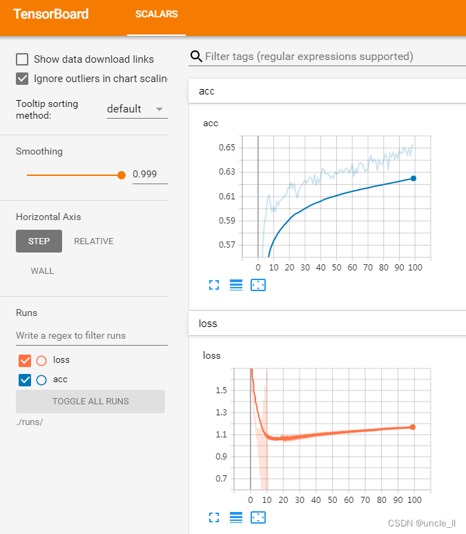
有些过拟合，可能是数据量太小，模型太大引起的。换成SMALL模型，效果为

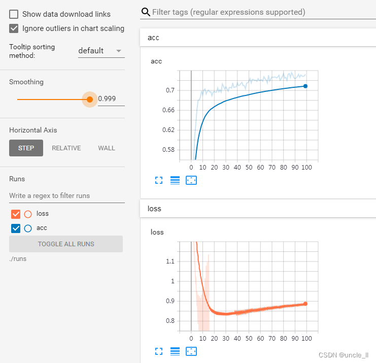
可以看到在cifar数据集的效果，相较于LARGE模型而言，SMALL模型更好一点

参考

• https://pytorch.org/vision/main/_modules/torchvision/models/mobilenetv3.html
• https://github.com/d-li14/mobilenetv3.pytorch
• https://github.com/leaderj1001/MobileNetV3-Pytorch
• https://blog.csdn.net/Chunfengyanyulove/article/details/91358187
• https://blog.csdn.net/thisiszdy/article/details/90167304
• https://www.cnblogs.com/wj-1314/p/12108424.html