


2024.01.13 过拟合解决方案之权重衰减
范数
线性代数中最有用的一些运算符是范数(norm)。 非正式地说,向量的范数是表示一个向量有多大。 这里考虑的大小(size)概念不涉及维度,而是分量的大小。
范数听起来很像距离的度量。 欧几里得距离和毕达哥拉斯定理中的非负性概念和三角不等式可能会给出一些启发。 事实上,欧几里得距离是一个
L
2
L_2
L2范数: 假设
n
n
n维向量
x
\mathbf{x}
x中的元素是
x
1
,
…
,
x
n
x_{1},\ldots,x_{n}
x1,…,xn,其
L
2
L_2
L2范数是向量元素平方和的平方根:
∥
x
∥
2
=
∑
i
=
1
n
x
i
2
,
\|\mathbf{x}\|_2=\sqrt{\sum_{i=1}^nx_i^2},
∥x∥2=i=1∑nxi2,
其中,在
L
2
L_2
L2范数中常常省略下标2,也就是说
∥
x
∥
\|\mathbf{x}\|
∥x∥等同于
∥
x
∥
2
\|\mathbf{x}\|_2
∥x∥2。在代码中,我们可以按如下方式计算向量的
L
2
L_2
L2范数。
u = torch.tensor([3.0, -4.0])
torch.norm(u)
输出:
tensor(5.)
深度学习中更经常地使用
L
2
L_2
L2范数的平方,也会经常遇到
L
1
L_1
L1范数,它表示为向量元素的绝对值之和:
∥
x
∥
1
=
∑
i
=
1
n
∣
x
i
∣
\|\mathbf{x}\|_1=\sum_{i=1}^n|x_i|
∥x∥1=i=1∑n∣xi∣
权重衰退原理
在训练参数化机器学习模型时, 权重衰减(weight decay)是最广泛使用的正则化的技术之一, 它通常也被称为 L 2 L_2 L2正则化。 这项技术通过函数与零的距离来衡量函数的复杂度。 但是我们应该如何精确地测量一个函数和零之间的距离呢? 没有一个正确的答案。 事实上,函数分析和巴拿赫空间理论的研究,都在致力于回答这个问题。
一种简单的方法是通过线性函数 f ( x ) = w ⊤ x f(\mathbf{x})=\mathbf{w}^\top\mathbf{x} f(x)=w⊤x中的权重向量的某个范数来度量其复杂性, 例如 ∥ w ∥ 2 \|\mathbf{w}\|^2 ∥w∥2。要保证权重向量比较小, 最常用方法是将其范数作为惩罚项加到最小化损失的问题中。 将原来的训练目标最小化训练标签上的预测损失, 调整为最小化预测损失和惩罚项之和。 现在,如果我们的权重向量增长的太大, 我们的学习算法可能会更集中于最小化权重范数 ∥ w ∥ 2 \|\mathbf{w}\|^2 ∥w∥2。这正是我们想要的。
例如线性回归的损失函数如下:
L
(
w
,
b
)
=
1
n
∑
i
=
1
n
1
2
(
w
⊤
x
(
i
)
+
b
−
y
(
i
)
)
2
L(\mathbf{w},b)=\frac1n\sum_{i=1}^n\frac12\Big(\mathbf{w}^\top\mathbf{x}^{(i)}+b-y^{(i)}\Big)^2
L(w,b)=n1i=1∑n21(w⊤x(i)+b−y(i))2
其中,
x
(
i
)
\mathbf{x}^{(i)}
x(i)是样本
i
i
i的特征,
y
(
i
)
{y}^{(i)}
y(i)是样本
i
i
i的标签,
(
w
,
b
)
(\mathbf{w},b)
(w,b)是权重和偏置参数。 为了惩罚权重向量的大小, 我们必须以某种方式在损失函数中添加
∥
w
∥
2
\|\mathbf{w}\|^2
∥w∥2,但是模型应该如何平衡这个新的额外惩罚的损失? 实际上,我们通过正则化常数
λ
\lambda
λ来描述这种权衡, 这是一个非负超参数,我们使用验证数据拟合:
L
(
w
,
b
)
+
λ
2
∥
w
∥
2
L(\mathbf{w},b)+\frac\lambda2\|\mathbf{w}\|^2
L(w,b)+2λ∥w∥2
对于
λ
=
0
\lambda = 0
λ=0,我们恢复了原来的损失函数。 对于
λ
>
0
\lambda > 0
λ>0,我们限制
∣
w
∥
|\mathbf{w}\|
∣w∥的大小。 这里我们仍然除以2,当我们取一个二次函数的导数时, 2和1/2会抵消,以确保更新表达式看起来既漂亮又简单。为什么在这里我们使用平方范数而不是标准范数(即欧几里得距离)? 我们这样做是为了便于计算。 通过平方
L
2
L_2
L2范数,我们去掉平方根,留下权重向量每个分量的平方和。 这使得惩罚的导数很容易计算。
L
2
L_2
L2正则化回归的小批量随机梯度下降更新如下式:
w
←
(
1
−
η
λ
)
w
−
η
∣
B
∣
∑
i
∈
B
x
(
i
)
(
w
⊤
x
(
i
)
+
b
−
y
(
i
)
)
\mathbf{w}\leftarrow(1-\eta\lambda)\mathbf{w}-\frac\eta{|\mathcal{B}|}\sum_{i\in\mathcal{B}}\mathbf{x}^{(i)}\left(\mathbf{w}^\top\mathbf{x}^{(i)}+b-y^{(i)}\right)
w←(1−ηλ)w−∣B∣ηi∈B∑x(i)(w⊤x(i)+b−y(i))
根据之前章节所讲的,我们根据估计值与观测值之间的差异来更新
w
\mathbf{w}
w。 然而,我们同时也在试图将
w
\mathbf{w}
w的大小缩小到零。 这就是为什么这种方法有时被称为权重衰减。 我们仅考虑惩罚项,优化算法在训练的每一步衰减权重。 与特征选择相比,权重衰减为我们提供了一种连续的机制来调整函数的复杂度。 较小的值对
λ
\lambda
λ应较少约束的
w
\mathbf{w}
w, 而较大的
λ
\lambda
λ值对
w
\mathbf{w}
w的约束更大。
从零开始实现权重衰退
1 构造数据
import torch
from torch import nn
from torch.utils import data


def synthetic_data(w, b, num_examples):
    """生成y=Xw+b+噪声"""
    X = torch.normal(0, 1, (num_examples, len(w)))
    y = torch.matmul(X, w) + b
    y += torch.normal(0, 0.01, y.shape)
    return X, y.reshape((-1, 1))


def load_array(data_arrays, batch_size, is_train=True):
    """构造一个PyTorch数据迭代器"""
    dataset = data.TensorDataset(*data_arrays)
    return data.DataLoader(dataset, batch_size, shuffle=is_train)


n_train, n_test, num_inputs, batch_size = 20, 100, 200, 5
true_w, true_b = torch.ones((num_inputs, 1)) * 0.01, 0.05
train_data = synthetic_data(true_w, true_b, n_train)
train_iter = load_array(train_data, batch_size)
test_data = synthetic_data(true_w, true_b, n_test)
test_iter = load_array(test_data, batch_size, is_train=False)
2 初始化模型参数
def init_params():
    w = torch.normal(0, 1, size=(num_inputs, 1), requires_grad=True)
    b = torch.zeros(1, requires_grad=True)
    return [w, b]
3 定义 L 2 {L}_2 L2范数惩罚
def l2_penalty(w):
    return torch.sum(w.pow(2)) / 2
4 定义模型和损失函数
def linreg(X, w, b):
    """线性回归模型"""
    return torch.matmul(X, w) + b


def squared_loss(y_hat, y):
    """均方损失"""
    return (y_hat - y.reshape(y_hat.shape)) ** 2 / 2


def sgd(params, lr, batch_size):
    """小批量随机梯度下降"""
    with torch.no_grad():
        for param in params:
            param -= lr * param.grad / batch_size
            param.grad.zero_()
5 定义损失评估函数
class Accumulator:  #@save
    """在n个变量上累加"""
    def __init__(self, n):
        self.data = [0.0] * n

    def add(self, *args):
        self.data = [a + float(b) for a, b in zip(self.data, args)]

    def reset(self):
        self.data = [0.0] * len(self.data)

    def __getitem__(self, idx):
        return self.data[idx]


def evaluate_loss(net, data_iter, loss):
    """评估给定数据集上模型的损失"""
    metric = Accumulator(2)  # 损失的总和,样本数量
    for X, y in data_iter:
        out = net(X)
        y = y.reshape(out.shape)
        l = loss(out, y)
        metric.add(l.sum(), l.numel())
    return metric[0] / metric[1]
6 定义训练函数
def train(lambd):
    w, b = init_params()
    net, loss = lambda X: linreg(X, w, b), squared_loss
    num_epochs, lr = 100, 0.003
    for epoch in range(num_epochs):
        for X, y in train_iter:
            # 增加了L2范数惩罚项,
            # 广播机制使l2_penalty(w)成为一个长度为batch_size的向量
            l = loss(net(X), y) + lambd * l2_penalty(w)
            l.sum().backward()
            sgd([w, b], lr, batch_size)
        if (epoch + 1) % 10 == 0:
            print(evaluate_loss(net, train_iter, loss))
            print(evaluate_loss(net, test_iter, loss))
    print('w的L2范数是:', torch.norm(w).item())
7 定义训练函数
def train(lambd):
    w, b = init_params()
    net, loss = lambda X: linreg(X, w, b), squared_loss
    num_epochs, lr = 100, 0.003
    for epoch in range(num_epochs):
        for X, y in train_iter:
            # 增加了L2范数惩罚项,
            # 广播机制使l2_penalty(w)成为一个长度为batch_size的向量
            l = loss(net(X), y) + lambd * l2_penalty(w)
            l.sum().backward()
            sgd([w, b], lr, batch_size)
        if (epoch + 1) % 10 == 0:
            print(evaluate_loss(net, train_iter, loss))
            print(evaluate_loss(net, test_iter, loss))
    print('w的L2范数是:', torch.norm(w).item())
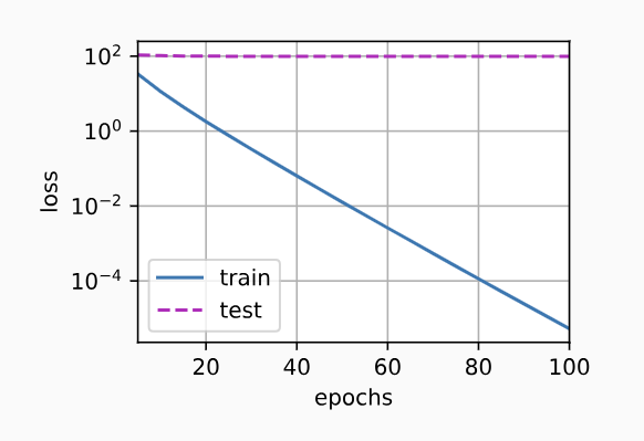
8 忽略正则化直接训练
我们现在用lambd = 0禁用权重衰减后运行这个代码。 注意,这里训练误差有了减少,但测试误差没有减少, 这意味着出现了严重的过拟合。
train(lambd=0)
输出:
6.718327045440674
111.89330017089844
0.769484794139862
110.775845413208
0.12477019131183624
110.69607948303222
0.023347004130482674
110.73360847473144
0.004730253014713526
110.76803649902344
0.0010142373736016451
110.78975273132325
0.0002265329472720623
110.80156417846679
5.242526312940754e-05
110.80791412353516
1.2483596856327495e-05
110.81120208740235
3.029539379895141e-06
110.8129093170166
w的L2范数是: 14.017784118652344
其图像如下:
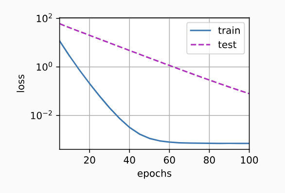
9 使用权重衰减
下面,我们使用权重衰减来运行代码。 注意,在这里训练误差增大,但测试误差减小。 这正是我们期望从正则化中得到的效果。
train(lambd=3)
输出:
3.4674706935882567
40.52239170074463
0.21071776300668715
19.59771007537842
0.017328211199492217
9.598615684509276
0.0028875970747321844
4.72015061378479
0.0016041443683207034
2.3360534596443174
0.0014270563377067446
1.169337533712387
0.001352554582990706
0.5967587316036225
0.0013034804665949195
0.31446478426456453
0.0012782146106474102
0.1743188387155533
0.0012224957521539182
0.103997398391366
w的L2范数是: 0.37360531091690063
图像:
权重衰退简洁实现
1 构造数据
import torch
from torch import nn
from torch.utils import data


def synthetic_data(w, b, num_examples):
    """生成y=Xw+b+噪声"""
    X = torch.normal(0, 1, (num_examples, len(w)))
    y = torch.matmul(X, w) + b
    y += torch.normal(0, 0.01, y.shape)
    return X, y.reshape((-1, 1))


def load_array(data_arrays, batch_size, is_train=True):
    """构造一个PyTorch数据迭代器"""
    dataset = data.TensorDataset(*data_arrays)
    return data.DataLoader(dataset, batch_size, shuffle=is_train)


n_train, n_test, num_inputs, batch_size = 20, 100, 200, 5
true_w, true_b = torch.ones((num_inputs, 1)) * 0.01, 0.05
train_data = synthetic_data(true_w, true_b, n_train)
train_iter = load_array(train_data, batch_size)
test_data = synthetic_data(true_w, true_b, n_test)
test_iter = load_array(test_data, batch_size, is_train=False)
2 定义损失评估函数
class Accumulator:  #@save
    """在n个变量上累加"""
    def __init__(self, n):
        self.data = [0.0] * n

    def add(self, *args):
        self.data = [a + float(b) for a, b in zip(self.data, args)]

    def reset(self):
        self.data = [0.0] * len(self.data)

    def __getitem__(self, idx):
        return self.data[idx]


def evaluate_loss(net, data_iter, loss):
    """评估给定数据集上模型的损失"""
    metric = Accumulator(2)  # 损失的总和,样本数量
    for X, y in data_iter:
        out = net(X)
        y = y.reshape(out.shape)
        l = loss(out, y)
        metric.add(l.sum(), l.numel())
    return metric[0] / metric[1]
3 定义训练函数
在下面的代码中,我们在实例化优化器时直接通过weight_decay指定weight decay超参数。 默认情况下,PyTorch同时衰减权重和偏移。 这里我们只为权重设置了weight_decay,所以偏置参数b不会衰减。
def train_concise(wd):
    net = nn.Sequential(nn.Linear(num_inputs, 1))
    for param in net.parameters():
        param.data.normal_()
    loss = nn.MSELoss(reduction='none')
    num_epochs, lr = 100, 0.003
    # 偏置参数没有衰减
    trainer = torch.optim.SGD([
        {"params":net[0].weight,'weight_decay': wd},
        {"params":net[0].bias}], lr=lr)
    for epoch in range(num_epochs):
        for X, y in train_iter:
            trainer.zero_grad()
            l = loss(net(X), y)
            l.mean().backward()
            trainer.step()
        if (epoch + 1) % 10 == 0:
            print(evaluate_loss(net, train_iter, loss))
            print(evaluate_loss(net, test_iter, loss))
    print('w的L2范数:', net[0].weight.norm().item())
4 忽略正则化直接训练
我们现在用lambd = 0禁用权重衰减后运行这个代码。 注意,这里训练误差有了减少,但测试误差没有减少, 这意味着出现了严重的过拟合。
train_concise(0)
输出:
0.7942435622215271
147.39787200927734
0.026174949016422033
147.1616212463379
0.0011757630854845047
147.12282012939454
5.728952528443188e-05
147.11509490966796
2.8377404078128167e-06
147.11357345581055
1.435657850379357e-07
147.11323837280273
7.450126027208626e-09
147.11319473266602
3.930717806799322e-10
147.11319717407227
4.2250853510283905e-11
147.1131950378418
1.3290707423507797e-11
147.1131904602051
w的L2范数: 13.41625690460205
其图像如下:
5 使用权重衰减
下面,我们使用权重衰减来运行代码。 注意,在这里训练误差增大,但测试误差减小。 这正是我们期望从正则化中得到的效果。
train_concise(3)
输出:
0.44908093512058256
79.26161060333251
0.014182116836309433
38.39419065475464
0.005516740120947361
18.69626650810242
0.0047397946938872336
9.167555465698243
0.004471739660948515
4.554769878387451
0.004199517332017422
2.32014231801033
0.004032817389816046
1.2366495299339295
0.003825438302010298
0.7090656226873397
0.003553233714774251
0.45032487854361536
0.003349584457464516
0.32078503906726835
w的L2范数: 0.3820874094963074
图像:
欢迎关注公众号


 515
515


 被折叠的 条评论
为什么被折叠?
被折叠的 条评论
为什么被折叠?
 到【灌水乐园】发言


