


It’s challenging to convert higher dimensional data to lower dimensions or visualize the data with hundreds of attributes or even more. Too many attributes lead to overfitting of data, thus results in poor prediction.
将较高维度的数据转换为较低维度或使用数百个甚至更多个属性可视化数据是一项挑战。 太多的属性导致数据过度拟合,从而导致不良的预测。
Dimensionality reduction is the best approach to deal with such data. A large number of attributes in dataset leads may lead to overfitting of datasets. There are several techniques for dimensionality reduction. The three popular dimensionality reduction techniques to identify the set of significant features and reduce dimensions of the dataset are
d imensionality减少处理此类数据的最佳方式。 数据集线索中的大量属性可能会导致数据集过拟合。 有几种降低尺寸的技术。 三种常见的降维技术可用于识别重要特征集并缩小数据集的维数,分别是
1) Principle Component Analysis (PCA)
1)主成分分析(PCA)
2) Linear Discriminant Analysis (LDA)
2)线性判别分析(LDA)
3) Kernel PCA (KPCA)
3)内核PCA(KPCA)
In this article, we are going to look into Fisher’s Linear Discriminant Analysis from scratch.
在本文中,我们将从头开始研究Fisher的线性判别分析。
LDA is a supervised linear transformation technique that utilizes the label information to find out informative projections. A proper linear dimensionality reduction makes our binary classification problem trivial to solve. In this classification, the dimensionality feature space is reduced to a 1-D dimension by projecting on the vector.
LDA是一种受监督的线性变换技术,该技术利用标签信息来找出信息丰富的投影。 适当的线性降维使得我们的二进制分类问题很难解决。 在该分类中,通过投影在矢量上,将维特征空间减小为一维维。
In this approach, we take the shadow of points along the line or hyperplane. Through visual inspection, we can tell that it is easy to classify these examples into two classes that are positive and negative if we project points into the projection direction labeled as “FLD” (the solid green line). After the projection, the positive class examples will clump into a small range of values, as do the negative examples. However, it must be ensured that the range of projected values in different classes never overlap.
在这种方法中,我们沿直线或超平面拍摄点的阴影。 通过目视检查,如果将点投影到标记为“ FLD” (绿色实线)的投影方向上,我们可以很容易地将这些示例分为正和负两类。 预测之后,正面类的例子将与一小部分数值相抵触,负面类也是如此。 但是,必须确保不同类别中的投影值范围不会重叠。
Projecting data from d-dimensions onto a line
将d维数据投影到一条线上
Given a set of the n-D dimension feature vector of x1, x2, x3……, xn.
给定一组x1,x2,x3……,xn的nD维特征向量。
We want to form a linear combination of the components of x as:
我们希望将x的分量形成线性组合,如下所示:
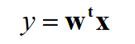
Where w denotes the direction of the FLD vector. There can be several values of w, as shown below (for binary classification)
其中w表示FLD矢量的方向。 w可以有多个值,如下所示(对于二进制分类)
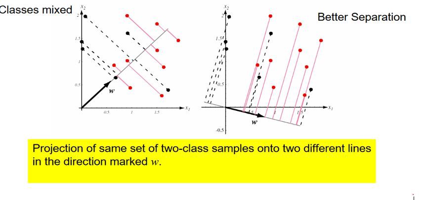
As you can see, for better separation, we need to find appropriate direction w. So, to find it let define two terms (for binary classification):
如您所见,为了更好地分离,我们需要找到合适的方向w。 因此,要找到它,请定义两个术语(用于二进制分类):
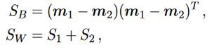
Here, m1-m2 is the mean difference between the two classes. SB is called the between-class scatter matrix, and SW is the within-class scatter matrix (both are D×D in size). SW measures how scattered is the original input dataset within each class. SB measures the scatter caused by the two-class means, which measures how scattered it is between different classes.
在此,m1-m2是两个类别之间的平均差。 SB被称为类间散布矩阵,SW被称为类内散布矩阵(大小均为D×D)。 SW衡量每个类中原始输入数据集的分散程度。 SB测量由两类方法导致的分散,这测量了它在不同类之间的分散程度。
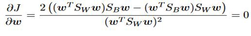
FLD objective function is given by J as:
FLD目标函数由J给出为:
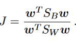
In other words, this optimization aims at finding a projection direction that makes the between-class scatter much larger than the within-class scatter. Finding the derivative of J with respect to w to maximize J, we get,
换句话说,此优化旨在寻找使类间散布比类内散布大得多的投影方向。 找到关于w的J的导数以最大化J,我们得到,
Hence, the necessary condition obtained for optimality is,
因此,获得最优性的必要条件是
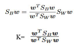
Here, K is a scalar value, which implies that w is a generalized eigenvector of SB and Sw, and K is the eigenvalue corresponding to it. Similarly, J is an optimization function and generalized eigenvalue. So, we need to maximize J w.r.t w to get the largest eigenvalue, thus getting the required projection direction, w.
在这里,K 是一个标量值,表示w是SB和Sw的广义特征向量,而K是与其对应的特征值。 同样,J是一个优化函数和广义特征值。 因此,我们需要最大化J wrt w以获得最大特征值,从而获得所需的投影方向w 。
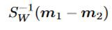
On solving the above optimality condition, the optimal projection direction (w) can be represented as
通过求解上述最优条件,可以将最优投影方向( w )表示为
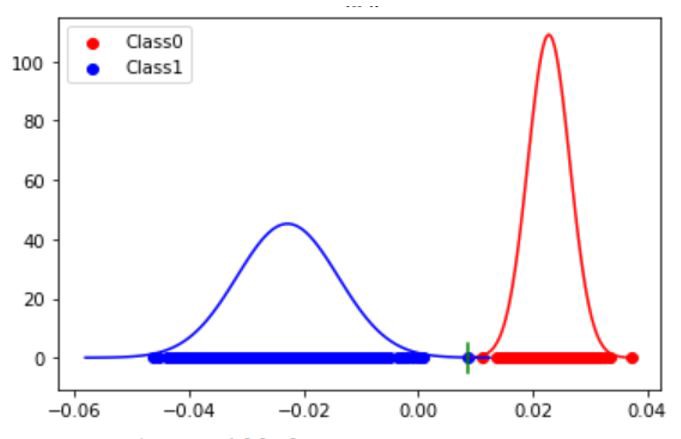
Thus, all the points get projected on the line in the direction of w for better separation. The projected data can subsequently be used to construct a discriminant by choosing a threshold y0. When y(x)>y*, the point will belong to class 1; otherwise, it will belong to class 0. In this case, the point y* is chosen as the intersection of the Gaussian standard distribution curve of the two classes.
因此,所有点都沿w方向投影在直线上,以实现更好的分离。 随后可以通过选择阈值y0将投影数据用于构造判别式。 当y(x)> y *时,该点属于1类;否则,该点属于1类。 否则,它将属于0类。在这种情况下,选择点y *作为两个类的高斯标准分布曲线的交点。
Implementation of FLD
FLD的实施
Using a dataset of 3 features for binary classification,
使用3个要素的数据集进行二进制分类,
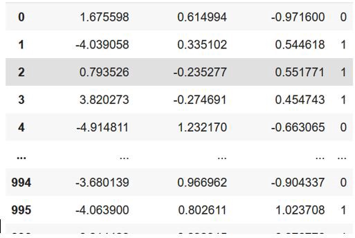
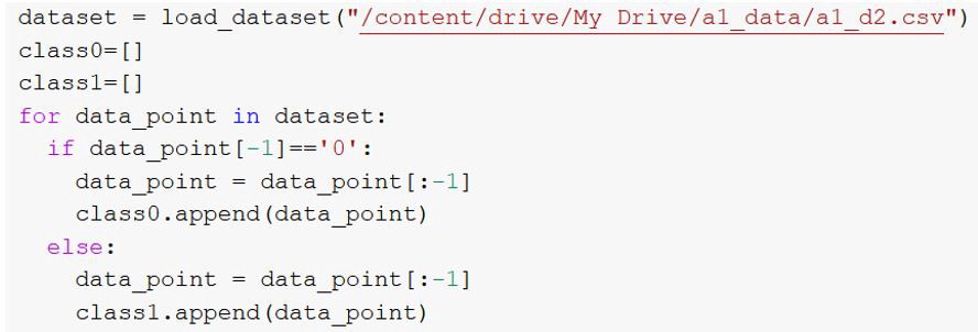
Firstly, split the dataset in Class 0 (c0) and Class 1 (c1) depending upon the Y actual.
首先,根据Y实际值将数据集分为Class 0(c0)和Class 1(c1)。
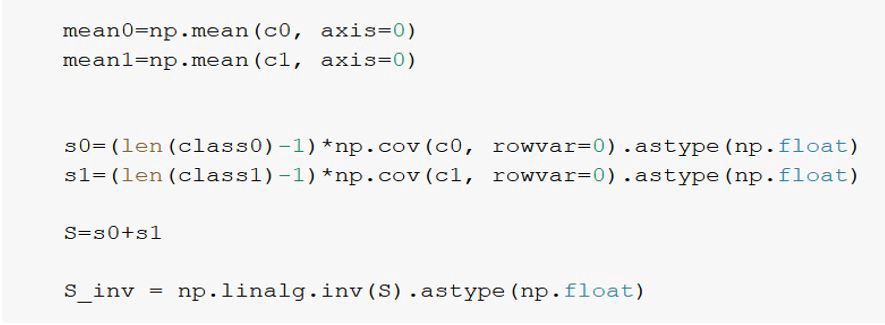
To find w, let’s calculate mean0 (c2 mean), mean1 (c1 mean), and S_inv (Sw^-1)
为了找到w,让我们计算均值0(c2均值),均值1(c1均值)和S_inv(Sw ^ -1)
Calculating w, y0, y1, where y0 and y1 are projections of points belonging to class 0 (c0) and class1 (c1) in the direction of w
计算w,y0,y1 ,其中y0和y1是属于类别0(c0)和类别1(c1)的点在w方向上的投影

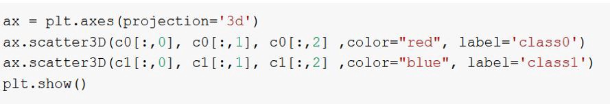
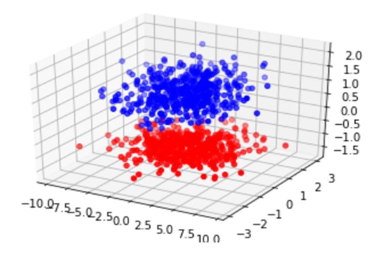
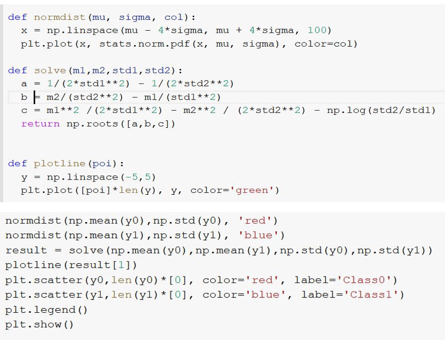
Plotting points belonging to class 0 and class 1,
绘制属于0类和1类的点
Normalizing the projected data and plotting it
归一化投影数据并作图
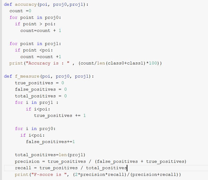
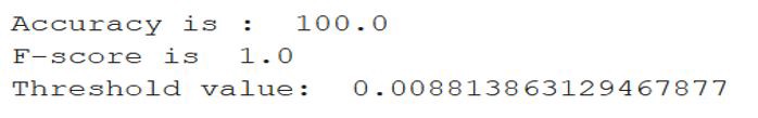
After making predictions of the above data through LDA, accuracy, and F-measure for the given data are:
通过LDA对上述数据进行预测后,给定数据的准确性和F度量为:
Above, implementation is done for binary classification, but an extension of the above algorithm is used to make predictions for multiclass classification.
上面,完成了用于二进制分类的实现,但是使用了上述算法的扩展来进行多类分类的预测。
Pat on your back for following the post so far and I hope you have fun while learning. Stay tuned for my next post
帕特(Pat)支持您关注到目前为止的帖子,希望您在学习时玩得开心。 请继续关注我的下一篇文章
Thank you for being here …. Happy Learning :)
非常感谢您的到来 …。 快乐学习:)
翻译自: https://medium.com/@priyankagupta_32252/fishers-linear-discriminant-analysis-a03baa603e89


 3623
3623


 被折叠的 条评论
为什么被折叠?
被折叠的 条评论
为什么被折叠?
 到【灌水乐园】发言


