分类模型评估指标_分类模型的评估指标系列第1部分

分类模型评估指标

The evaluation metrics for classification models series consist of multiple articles linked together geared to teaching you the best practices in evaluating classification model performance.

分类模型评估指标系列由多篇文章链接在一起，旨在教您评估分类模型性能的最佳实践。

For our practice example, we’ll be using the breast cancer dataset available through “sklearn”. We take the following steps in preparing our data:

对于我们的实践示例，我们将使用可通过“ sklearn”获得的乳腺癌数据集。 我们采取以下步骤来准备数据：

Next, we will proceed to split our data and train a binary classification model to evaluate.

接下来，我们将继续拆分数据并训练一个二进制分类模型进行评估。

We will create a table called evaluation_table with the actual and predicted values.

我们将创建一个包含实际值和预测值的表Evaluation_table。

We look up the percent of malignant vs benign observations.

我们查询了恶性与良性观察的百分比。

By looking at the percent of total observations in our sample that have actual (real) malignant cancer vs the percent that have benign, we analyze how balanced our sample truly is.

通过查看样本中有实际(实际)恶性肿瘤的总观察值与良性肿瘤的百分比，我们可以分析样本的真实平衡程度。

The imbalance we are dealing with is truly just 65:35. It is slightly imbalanced but is not of much concern. In a future article, I’ll be illustrating how to deal with highly imbalanced datasets.

我们正在处理的失衡确实只有65:35。 它有些不平衡，但并没有太大的问题。 在以后的文章中，我将说明如何处理高度不平衡的数据集。

Accuracy:

准确性：

The proportion of the observations that were predicted correctly.

正确预测的观测值所占的比例。

Accuracy is viable to use when the dataset has enough positive and negative observations. In this example, it is a viable metric to use because we have 65% malignant and 35% benign).

当数据集具有足够的正负观测值时，可以使用准确性。 在此示例中，这是可行的指标，因为我们有65％的恶性和35％的良性。

Accuracy stops being a viable evaluation metric when we have an ‘imbalanced dataset’, this is a dataset with considerably more negative than positive values or with considerably more positive than negative values.

当我们有一个“不平衡数据集”时，准确性就不再是可行的评估指标，这是一个负数比正值大得多或正数比负值大得多的数据集。

why?

为什么？

because the model will likely predict almost all the observations to be positive (or negative — depending on the direction of the imbalance), and be correct in most cases. If this happens The model will have a high accuracy regardless of its performance predicting the less represented negative (or positive) observations.

因为该模型可能会预测几乎所有观察结果都是积极的(或消极的，取决于失衡的方向)，并且在大多数情况下是正确的。 如果发生这种情况，则模型将具有较高的准确性，无论其性能如何预测较少代表的负面(或正面)观察。

Thresholds:

阈值：

We can set our binary classifier model to predict a probability instead of an integer. We do this by using the predict_proba() method of our model instead of predict().

我们可以将二进制分类器模型设置为预测概率而不是整数。 我们通过使用模型的predict_proba()方法而不是predict()来实现。

The result from using predict_proba() will be a 2D array with two columns: the probability of the cancer being benign, and the probability of the cancer is malignant. They should add up to 1 when summed. In order the check the order of the columns in the resulting array, we look up the clf.classes_ method.

使用predict_proba()的结果将是一个具有两列的二维数组：癌症良性的概率和癌症恶性的概率。 相加后，它们的总和应为1。 为了检查结果数组中列的顺序，我们查找clf.classes_方法。

We will be creating a column in our already existing evaluation data frame with the probability of the cancer being malignant (the second column of our array).

我们将在我们现有的评估数据框中创建一列，显示癌症为恶性的可能性(数组的第二列)。

When we begin prediction using the probability of an event taking place instead of looking at a binary prediction, we have the flexibility of choosing the probability threshold to be the cutoff point between 0 and 1. The ideal cutoff point will vary depending on the problem statement at hand, and the business needs the model is looking to solve.

当我们使用事件发生的概率开始预测而不是查看二进制预测时，我们可以灵活地选择概率阈值作为0到1之间的临界点。理想的临界点将根据问题陈述而有所不同。以及模型正在寻求解决的业务需求。

For example, if the benefit of a True Positive is large, and the cost of a False Positive is low, there would be more benefit in choosing a low cutoff point (example 0.2, 0.3) than to choose a high cutoff point (example 0.7, 0.8).

例如，如果“真阳性”的收益很大，而“假阳性”的成本很低，那么选择低截止点(例如0.2、0.3)比选择高截止点(例如0.7)会有更多的好处。 ，0.8)。

Nevertheless, to more easily compare the performance of two models, we want an evaluation metric that works independently from the chosen cutoff point.

但是，为了更轻松地比较两个模型的性能，我们需要一种评估指标，该指标独立于所选的临界点运行。

ROC，AUC和Gini： (ROC, AUC, and Gini:)

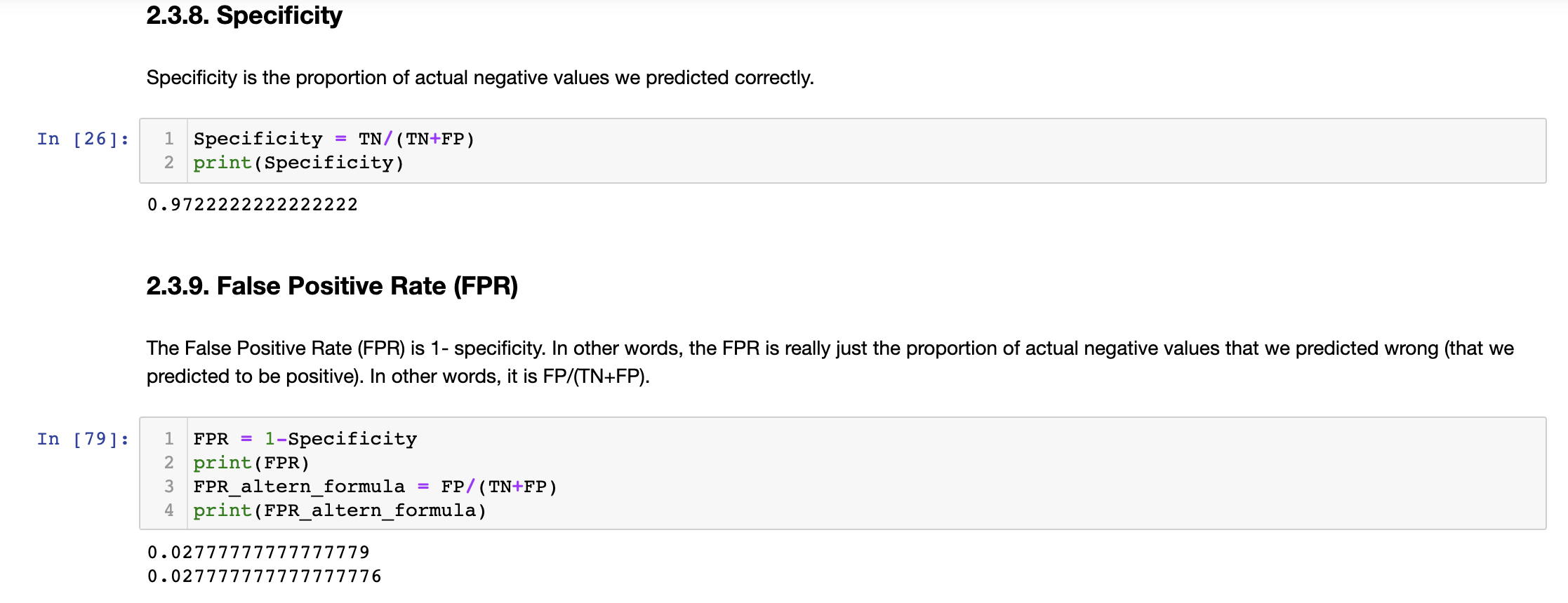
The ROC curve plots the relationship between the True Positive Rate (Precision) and the False Positive Rate (1-Specificity). In other words, we are comparing the proportion of correctly predicted positive observations (TP/(FP+TP)) vs the proportion of negative observations that were wrongly predicted (FP/(TN+FP)).

ROC曲线绘制了真实阳性率(精确度)和错误阳性率(1-特异性)之间的关系。 换句话说，我们正在比较正确预测的积极观察的比例(TP /(FP + TP))与错误预测的负面观察的比例(FP /(TN + FP))。

why?

为什么？

Because the ideal model would outperform other models by having a higher Precision (TPR), given the FPR (proportion of negative values that were wrongly predicted positive), regardless of the chosen threshold.

由于理想模型将通过具有更高的精度(TPR)而胜过其他模型，因此无论选择的阈值如何，在给定FPR(错误地预测为负的负值的比例)的情况下。

If we choose a threshold of 0.80, a higher number of observations will be predicted negative (predicted 0 — predicted that the cancer is benign). This would be that a higher proportion of the actual negative values is being predicted correctly (because at that threshold we are predicting a larger number of observations to be negative). This translates into a low FPR because the proportion of wrongly predicted actual negative values (predicted to be malignant/positive/1, but that was actually benign/negative/0) becomes lower.

如果我们将阈值设置为0.80，则将有更多的观察结果被预测为阴性(预测为0 －预测癌症是良性的)。 这可能是正确预测了较大比例的实际负值(因为在此阈值下，我们预测会有更多的观测值为负值)。 这意味着FPR较低，因为错误预测的实际负值(预测为恶性/阳性/ 1，但实际上是良性/阴性/ 0)的比例会降低。

Likewise, if we chose a lower threshold (example 0.20), we have the opposite effect. A higher proportion of the observations are being predicted positive/malignant/1, and therefore we have a higher FPR (a higher proportion of actual negative/benign/0 observations being wrongly predicted as positive/malignang/1).

同样，如果选择较低的阈值(例如0.20)，则效果相反。 较高比例的观察值被预测为阳性/恶性/ 1，因此我们的FPR较高(实际阴性/良性/ 0观察值中较高的比例被错误地预测为阳性/恶性肿瘤/ 1)。

The AUC is the area under the ROC curve. The higher the area under the curve the better the predictions are. Among the advantages of using this metric we find: — It comparable across models of different sample scales (it speaks in proportions of the sample) — It offers a comparison across models regardless of the chosen threshold

AUC是ROC曲线下的面积。 曲线下的面积越大，预测越好。 使用此度量标准的优势包括：-在不同样本比例的模型之间具有可比性(以样本的比例表示)-不管选择的阈值如何，都可以在模型之间进行比较

#This is my jupyter notebook with the information

翻译自: https://medium.com/swlh/evaluation-metrics-for-classification-models-series-part-1-88ea1cd80a88

分类模型评估指标