二维张量 乘以 三维张量_如何使用张量流实现线性回归

二维张量 乘以 三维张量

机器学习 (Machine Learning)

Let’s first briefly recall what linear regression is:

让我们首先简要回顾一下线性回归是什么：

Linear regression is estimating an unknown variable in a linear fashion by some other known variables. Visually, we fit a line (or a hyperplane in higher dimensions) through our data points.

线性回归是通过一些其他已知变量以线性方式估计未知变量。 在视觉上，我们通过数据点拟合一条线(或较大尺寸的超平面)。

If you’re not comfortable with this concept or want to understand better the math behind it, you can read my previous article about linear regression:

如果您对这个概念不满意，或者想更好地理解其背后的数学运算，可以阅读我以前关于线性回归的文章：

Probably, implementing linear regression with TensorFlow is an overkill. This library was made for more complicated stuff like neural networks, complex deep learning architectures, etc. Nevertheless, I think that using it for implementing a simpler machine learning method, like linear regression, is a good exercise for those who want to know how to build custom things with TensorFlow.

用TensorFlow实施线性回归可能是一个过大的杀伤力。 该库是为更复杂的东西(例如神经网络，复杂的深度学习体系结构等)制作的。尽管如此，我认为，将其用于实现更简单的机器学习方法(如线性回归)对于那些想知道如何使用TensorFlow构建自定义的东西。

TensorFlow has many APIs; and most introductory courses/tutorials only explain a higher-level API, like Keras. But that may not be sufficient, for example, if you want to use custom loss and/or activation functions that are not yet implemented in Keras.

TensorFlow有许多API。 并且大多数入门课程/教程仅介绍了Keras等高级API。 但这可能还不够，例如，如果您要使用Keras中尚未实现的自定义丢失和/或激活功能。

At its core, TensorFlow is just a math library similar to NumPy, but with 2 important improvements:

TensorFlow的核心只是一个类似于NumPy的数学库，但有两个重要的改进：

• It uses GPU to make its operations a lot faster. If you have a compatible GPU properly configured, TF 2 will automatically use it; no code changes are required.
  它使用GPU使其操作更快。 如果您具有正确配置的兼容GPU，则TF 2将自动使用它；否则，将自动使用它。 无需更改代码。
• It is capable of automatic differentiation; this means that for gradient-based methods you don’t need to manually compute the gradient, TensorFlow will do it for you.
  具有自动区分能力； 这意味着对于基于梯度的方法，您无需手动计算梯度，TensorFlow会为您完成。

You can think of TensorFlow as NumPy on steroids.

您可以将TensorFlow视为类固醇上的NumPy。

While these 2 features may not seem like big improvements for what we want to do here (linear regression), since this is not very computationally-expensive and the gradient is quite simple to compute manually, they make a big difference in deep learning where we need a lot of computing power and the gradient is quite nasty to calculate by hand.

尽管这两个功能似乎对我们在此处想要做的事情(线性回归)似乎没有很大的改进，但是由于这在计算上不是很昂贵，并且梯度很容易手动计算，因此它们在深度学习中有很大的不同需要大量的计算能力，并且手工计算梯度非常麻烦。

Now, let’s jump to the implementation.

现在，让我们跳到实现。

Firstly, we need to, obviously, import some libraries. We import tensorflow as it is the main thing we use for the implementation, matplotlib for visualizing our results, make_regression function, from sklearn, which we will be using to generate a regression dataset for using as an example, and the python’s built-in math module.

首先，显然，我们需要导入一些库。 我们导入tensorflow因为它是实现的主要内容，从matplotlib可视化结果，从sklearn make_regression函数，我们将使用它生成一个回归数据集作为示例，以及python的内置math函数模块。

import tensorflow as tfimport matplotlib.pyplot as pltfrom sklearn.datasets import make_regressionimport math

Then we will create a LinearRegression class with the following methods:

然后，我们将使用以下方法创建LinearRegression类：

• .fit() — this method will do the actual learning of our linear regression model; here we will find the optimal weights

  .fit() -此方法将实际学习我们的线性回归模型； 在这里我们将找到最佳权重

• .predict() — this one will be used for prediction; it will return the output of our linear model

  .predict() -这将用于预测； 它将返回线性模型的输出

• .rmse() — computes the root mean squared error of our model with the given data; this metric is kind of “the average distance from our model’s estimate to the true y value”

  .rmse() —使用给定数据计算模型的均方根误差； 该指标是“从模型估计值到真实y值的平均距离”

The first thing we do inside .fit() is to concatenate an extra column of 1’s to our input matrix X. This is to simplify our math and treat the bias as the weight of an extra variable that’s always 1.

我们在.fit()内部做的第一件事是将一个额外的1列连接到我们的输入矩阵X。这是为了简化我们的数学并将偏见视为额外变量的权重始终为1。

The .fit() method will be able to learn the parameters by using either closed-form formula or stochastic gradient descent. And to choose which to use, we will have a parameter called method that will expect a string of either ‘solve’ or ‘sgd’.

.fit()方法将能够通过使用闭式公式或随机梯度下降来学习参数。 为了选择使用哪个参数，我们将有一个名为method的参数，该参数期望使用'solve'或'sgd'的字符串。

When method is set to ‘solve’ we will get the weights of our model by the following formula:

当method设置为“ solve”时，我们将通过以下公式获得模型的权重：

which requires the matrix X to have full column rank; so, we will check for this and otherwise we show an error message.

这要求矩阵X具有完整的列等级； 因此，我们将对此进行检查，否则将显示错误消息。

The first part of our .fit() method is:

我们的.fit()方法的第一部分是：

def fit(self, X, y, method, learning_rate=0.01, iterations=500, batch_size=32):
    X = tf.concat([X, tf.ones_like(y, dtype=tf.float32)], axis=1)
    rows, cols = X.shape
    if method == 'solve':
        if rows >= cols == tf.linalg.matrix_rank(X):
            self.weights = tf.linalg.matmul(
                tf.linalg.matmul(
                    tf.linalg.inv(
                        tf.linalg.matmul(
                            X,
                            X, transpose_a=True)),
                    X, transpose_b=True),
                y)
        else:
            print('X has not full column rank. method=\'solve\' cannot be used.')

Note that the other parameters after method are optional and are used only in the case we use SGD.

请注意， method之后的其他参数是可选的，仅在使用SGD的情况下使用。

The second part of this method handles the case of method = ‘sgd’, which doesn’t require that X has full column rank.

此方法的第二部分处理method = 'sgd'的情况，该方法不需要X具有完整的列等级。

The SGD algorithm for our least squares linear regression is sketched below:

下面概述了用于最小二乘线性回归的SGD算法：

We will start this algorithm by initializing the weights class attribute to a TensorFlow Variable which is a column vector with values drawn from a normal distribution with mean 0 and standard deviation 1/(number of columns). We divide the standard deviation by the number of columns to make sure we don’t get too big values as output in the initial stages of the algorithm. This is to help us converge faster.

我们将通过将权重类属性初始化为TensorFlow变量来启动此算法，TensorFlow变量是一个列向量，其值取自均值0和标准差1 /(列数)的正态分布。 我们将标准偏差除以列数，以确保在算法的初始阶段不会得到太大的输出值。 这是为了帮助我们更快地收敛。

At the beginning of each iteration, we randomly shuffle our rows of data. Then, for each batch, we compute the gradient and subtract it (multiplied by the learning rate) from the current weights vector to obtain the new weights.

在每次迭代的开始，我们随机地随机整理数据行。 然后，对于每个批次，我们计算梯度并将其从当前权重向量中减去(乘以学习率)以获得新的权重。

In the SGD algorithm sketched above, we had shown the manually computed gradient; it’s that expression multiplied by alpha (the learning rate). But in the code below we won’t compute that expression explicitly; instead, we compute the loss value:

在上面概述的SGD算法中，我们展示了手动计算的梯度。 就是表达式乘以alpha(学习率)。 但是在下面的代码中，我们不会显式地计算该表达式； 相反，我们计算损失值：

then we let TensorFlow compute the gradient for us.

然后让TensorFlow为我们计算梯度。

Below is the second half of our .fit() method:

以下是我们的.fit()方法的.fit() ：

elif method == 'sgd':
        self.weights = tf.Variable(tf.random.normal(stddev=1.0/cols, shape=(cols, 1)))
        for i in range(iterations):
            Xy = tf.concat([X, y], axis=1)
            Xy = tf.random.shuffle(Xy)
            X, y = tf.split(Xy, [Xy.shape[1]-1, 1], axis=1)
            for j in range(int(math.ceil(rows/batch_size))):
                begin, size = batch_size*j, batch_size if batch_size*(j+1) < rows else -1
                Xb, yb = tf.slice(X, [begin, 0], [size, -1]), tf.slice(y, [begin, 0], [size, -1])
                
                with tf.GradientTape() as tape:
                    diff = tf.math.subtract(
                        tf.linalg.matmul(Xb, self.weights),
                        yb)
                    loss_value = tf.linalg.matmul(diff, diff,
                                                    transpose_a=True)
                    
                gradient = tape.gradient(loss_value, self.weights)
                self.weights.assign_sub(
                    tf.multiply(learning_rate, gradient))
    else:
        print(f'Unknown method: \'{method}\'')
    
    return self

We need to compute the loss value inside the with tf.GradientTape() as tape block, then call tape.gradient(loss_value, self.weights) to get the gradient. For this to work, it is important that the quantity with respect to which the gradient is taken (self.weights) to be a tf.Variable object. Also, we should use the .assign_sub() method instead of -= when changing the weights.

我们需要with tf.GradientTape() as tape块计算出内部的损失值，然后调用tape.gradient(loss_value, self.weights)获得梯度。 为此，重要的是，将与之相对应的渐变量( self.weights )设为tf.Variable对象。 另外，更改权重时，应使用.assign_sub()方法而不是-= 。

We return self from this method to be able to concatenate the calls of the constructor and .fit() like this: lr = LinearRegression().fit(X, y, ‘solve’).

我们从此方法返回self ，以便能够像下面这样串联构造函数和.fit()的调用： lr = LinearRegression().fit(X, y, 'solve') 。

The .predict() method is quite straight-forward. We first check if .fit() was called before, then concatenate a column of 1’s to X and verify that the shape of X allows multiplication with the weights vector. If everything is OK, we simply return the result of the multiplication between X and the weights vector as the predictions.

.predict()方法非常简单。 我们首先检查是否曾经调用过.fit() ，然后将1的列连接到X并验证X的形状是否允许与权重向量相乘。 如果一切正常，我们只需返回X与权重向量之间相乘的结果作为预测。

def predict(self, X):
    if not hasattr(self, 'weights'):
        print('Cannot predict. You should call the .fit() method first.')
        return
    
    X = tf.concat([X, tf.ones((X.shape[0], 1), dtype=tf.float32)], axis=1)
    
    if X.shape[1] != self.weights.shape[0]:
        print(f'Shapes do not match. {X.shape[1]} != {self.weights.shape[0]}')
        return
    
    return tf.linalg.matmul(X, self.weights)

In .rmse() we first get the outputs of the model using .predict(), then if there were no errors during predict, we compute and return the root mean squared error which can be thought of as “the average distance from our model’s estimate to the true y value”.

在.rmse()我们首先使用得到了模型的输出.predict()然后如果有预测过程中没有错误，我们计算并返回这可以从我们的模型被认为是“平均距离的均方根误差估算到真正的y值”。

def rmse(self, X, y):
    y_hat = self.predict(X)
    
    if y_hat is None:
        return
    
    return tf.math.sqrt(
        tf.math.reduce_mean(
            tf.math.pow(tf.math.subtract(y_hat, y), 2)))

Below is the full code of the LinearRegression class:

下面是LinearRegression类的完整代码：

class LinearRegression:
    def fit(self, X, y, method, learning_rate=0.01, iterations=500, batch_size=32):
        X = tf.concat([X, tf.ones_like(y, dtype=tf.float32)], axis=1)
        rows, cols = X.shape
        if method == 'solve':
            if rows >= cols == tf.linalg.matrix_rank(X):
                self.weights = tf.linalg.matmul(
                    tf.linalg.matmul(
                        tf.linalg.inv(
                            tf.linalg.matmul(
                                X,
                                X, transpose_a=True)),
                        X, transpose_b=True),
                    y)
            else:
                print('X has not full column rank. method=\'solve\' cannot be used.')
        elif method == 'sgd':
            self.weights = tf.Variable(tf.random.normal(stddev=1.0/cols, shape=(cols, 1)))
            for i in range(iterations):
                Xy = tf.concat([X, y], axis=1)
                Xy = tf.random.shuffle(Xy)
                X, y = tf.split(Xy, [Xy.shape[1]-1, 1], axis=1)
                for j in range(int(math.ceil(rows/batch_size))):
                    begin, size = batch_size*j, batch_size if batch_size*(j+1) < rows else -1
                    Xb, yb = tf.slice(X, [begin, 0], [size, -1]), tf.slice(y, [begin, 0], [size, -1])
                    
                    with tf.GradientTape() as tape:
                        diff = tf.math.subtract(
                            tf.linalg.matmul(Xb, self.weights),
                            yb)
                        loss_value = tf.linalg.matmul(diff, diff,
                                                      transpose_a=True)
                        
                    gradient = tape.gradient(loss_value, self.weights)
                    self.weights.assign_sub(
                        tf.multiply(learning_rate, gradient))
        else:
            print(f'Unknown method: \'{method}\'')
        
        return self
    
    def predict(self, X):
        if not hasattr(self, 'weights'):
            print('Cannot predict. You should call the .fit() method first.')
            return
        
        X = tf.concat([X, tf.ones((X.shape[0], 1), dtype=tf.float32)], axis=1)
        
        if X.shape[1] != self.weights.shape[0]:
            print(f'Shapes do not match. {X.shape[1]} != {self.weights.shape[0]}')
            return
        
        return tf.linalg.matmul(X, self.weights)
    
    def rmse(self, X, y):
        y_hat = self.predict(X)
        
        if y_hat is None:
            return
        
        return tf.math.sqrt(
            tf.math.reduce_mean(
                tf.math.pow(tf.math.subtract(y_hat, y), 2)))

在示例中使用我们的LinearRegression类 (Using our LinearRegression class in an example)

To show our implementation of linear regression in action, we will generate a regression dataset with the make_regression() function from sklearn.

为了表示我们的实施行动线性回归，我们会生成一个数据集的回归与make_regression()从功能sklearn 。

X, y = make_regression(n_features=1, n_informative=1,
                       bias=1, noise=35)

Let’s plot this dataset to see how it looks like:

让我们绘制该数据集以查看其外观：

plt.scatter(X, y)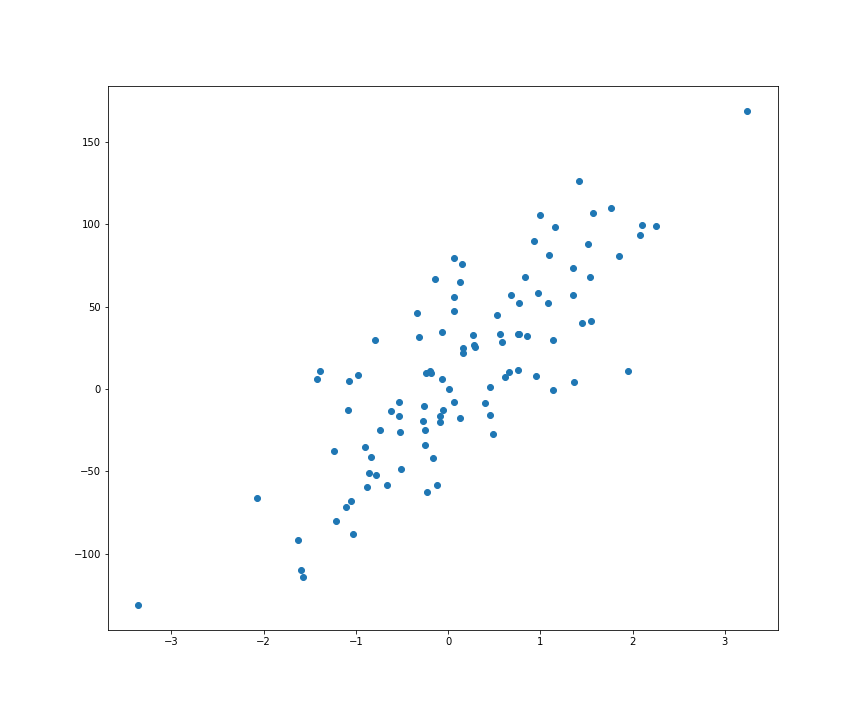

Image by Author

图片作者

The y returned by make_regression() is a flat vector. We will reshape it to a column vector to use with our LinearRegression class.

make_regression()返回的y是一个平面向量。 我们将其LinearRegression为列向量，以与LinearRegression类一起使用。

y = y.reshape((-1, 1))

Firstly, we will use method = ‘solve’ to fit the regression line:

首先，我们将使用method = 'solve'来拟合回归线：

lr_solve = LinearRegression().fit(X, y, method='solve')plt.scatter(X, y)plt.plot(X, lr_solve.predict(X), color='orange')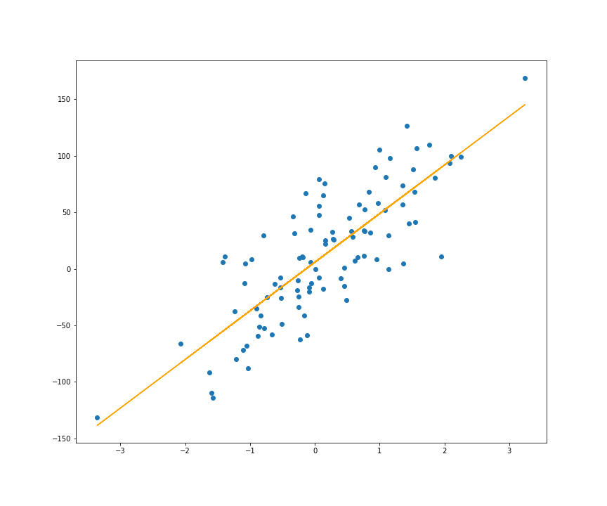

Image by Author

图片作者

The root mean squared error of the above regression model is:

上述回归模型的均方根误差为：

lr_solve.rmse(X, y)
# <tf.Tensor: shape=(), dtype=float32, numpy=37.436085>

Then, we also use method = ‘sgd’ and we will let the other parameters have their default values:

然后，我们还使用method = 'sgd' ，让其他参数具有其默认值：

lr_sgd = LinearRegression().fit(X, y, method='sgd')plt.scatter(X, y)plt.plot(X, lr_sgd.predict(X), color='orange')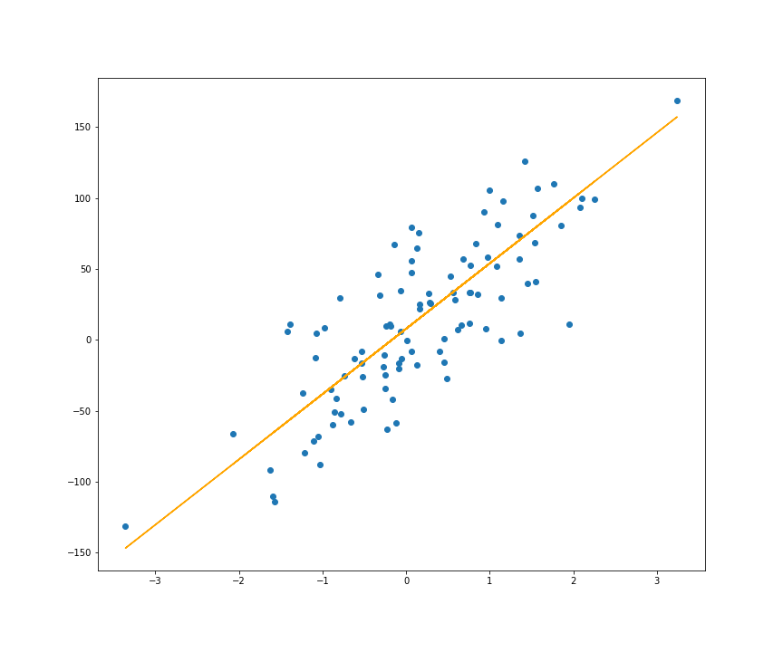

Image by Author

图片作者

As you can see, the regression lines in the 2 images above for methods ‘solve’ and ‘sgd’ are almost identical.

如您所见，上面两个图像中方法“ solve”和“ sgd”的回归线几乎相同。

The root mean squared error we got when using ‘sgd’ is:

使用'sgd'时得到的均方根误差为：

lr_sgd.rmse(X, y)
# <tf.Tensor: shape=(), dtype=float32, numpy=37.86531>

Here is the Jupyter Notebook with all the code:

这是Jupyter Notebook的所有代码：

I hope you found this information useful and thanks for reading! If you liked this article please consider following me on Medium to get my latest articles.

我希望您发现此信息有用，并感谢您的阅读！ 如果您喜欢这篇文章，请考虑在Medium上关注我，以获取我的最新文章。

翻译自: https://medium.com/towards-artificial-intelligence/how-to-implement-linear-regression-with-tensorflow-406b2cff1ffa

二维张量 乘以 三维张量