动量策略 python_在Python中使用动量通道进行交易

动量策略 python

Most traders use Bollinger Bands. However, price is not normally distributed. That’s why only 42% of prices will close within one standard deviation. Please go ahead and read this article. However, I have some good news.

大多数交易者使用布林带。 但是，价格不是正态分布的。 这就是为什么只有42％的价格会在一个标准偏差之内收盘的原因。 请继续阅读本文 。 但是，我有一些好消息。

Price is not normally distributed. Returns are!

价格不是正态分布。 退货都是！

Yes price is not normally distributed. Because price is nothing but sum of returns. And returns are normally distributed. So let’s jump in coding and hopefully you will have an “Aha!” moment.

是的，价格不是正态分布。 因为价格不过是回报之和。 收益是正态分布的。 因此，让我们开始编码，希望您会得到一个“ 啊哈 ！” 时刻。

I’m going to use EURUSD daily chart in my sample. However, it’s going to work with all assets and all timeframes.

我将在示例中使用EURUSD每日图表。 但是，它将适用于所有资产和所有时间范围。

Add required libraries

添加所需的库

# we only need these 3 libraries
import pandas as pd
import numpy as np
import matplotlib.pyplot as plt

Not let’s write the code to load our time-series dataset

不让我们编写代码来加载时间序列数据集

def load_file(f):
    fixprice = lambda x: float(x.replace(',', '.'))
    df = pd.read_csv(f)
    if "Gmt time" in df.columns:
        df['Date'] = pd.to_datetime(df['Gmt time'], format="%d.%m.%Y %H:%M:%S.%f")
    elif "time" in df.columns:
        df['Date'] = pd.to_datetime(df['time'], unit="s")
        df['Date'] = df['Date'] + np.timedelta64(3 * 60, "m")
        df[['Date', 'Open', 'High', 'Low', 'Close']] = df[['Date', 'open', 'high', 'low', 'close']]
        df = df[['Date', 'Open', 'High', 'Low', 'Close']]
    elif "Tarih" in df.columns:
        df['Date'] = pd.to_datetime(df['Tarih'], format="%d.%m.%Y")
        df['Open'] = df['Açılış'].apply(fixprice)
        df['High'] = df['Yüksek'].apply(fixprice)
        df['Low'] = df['Düşük'].apply(fixprice)
        df['Close'] = df['Şimdi'].apply(fixprice)
    else:
        df["Date"] = pd.to_datetime(df["Date"])
    # we need to shift or we will have lookahead bias in code
    df["Returns"] = (df["Close"].shift(1) - df["Close"].shift(2)) / df["Close"].shift(2)
    return df

Now if you look at the code, I have added a column “Returns” and it’s shifted. We don’t want our indicator to repaint and i don’t want to have lookahead bias. I am basically calculating the change from yesterday’s close to today’s close and shifting.

现在，如果您看一下代码，我添加了“ Returns”列，它已转移。 我们不希望我们的指标重新粉刷，我也不想有前瞻性偏见。 我基本上是在计算从昨天的收盘价到今天的收盘价的变化。

Load your dataset and plot histogram of Returns

加载数据集并绘制退货的直方图

sym = "EURUSD"
period = "1d"
fl = "./{YOUR_PATH}/{} {}.csv".format(period, sym)
df = load_file(fl)
df["Returns"].hist(bins=1000, grid=False)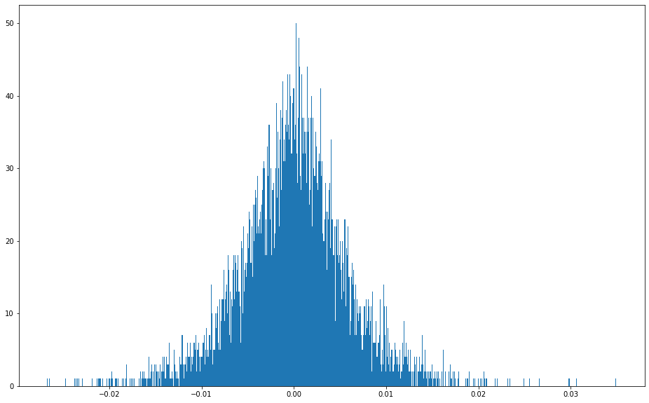

EURUSD daily returns histogram

EURUSD每日收益柱状图

Perfect bell shape curve. Now we know that we can get some real probabilities right? Empirical Rule (a.k.a. 68–95–99.7 rule) states that 68% of data will fall within one standard deviation, 95% of data will fall within two standard deviation and 99.7% of data will fall within three standard deviation. Ok let’s write the code to calculate it for us.

完美的钟形曲线。 现在我们知道可以得到一些真实的概率了吗？ 经验法则 (也称为68–95–99.7规则)指出，68％的数据将落在一个标准偏差内，95％的数据将落在两个标准偏差内，而99.7％的数据将落在三个标准偏差内。 好的，让我们编写代码为我们计算一下。

def add_momentum(df, lb=20, std=2):
    df["MA"] = df["Returns"].rolling(lb).mean()
    df["STD"] = df["Returns"].rolling(lb).std()
    df["OVB"] = df["Close"].shift(1) * (1 + (df["MA"] + df["STD"] * std))
    df["OVS"] = df["Close"].shift(1) * (1 + (df["MA"] - df["STD"] * std))
    return df

Now as we already have previous Bar’s close, it’s easy and safe to use and calculate the standard deviation. Also it’s easy for us to have overbought and oversold levels in advance. And they will stay there from the beginning of the current period. I also want to be sure if my data going to follow the empirical rule. So i want to get the statistics. Let’s code that block as well.

现在，由于我们已经关闭了先前的Bar，因此可以轻松安全地使用和计算标准偏差。 同样，我们很容易提前超买和超卖。 他们将从当前阶段开始一直呆在那里。 我还想确定我的数据是否遵循经验法则。 所以我想获得统计数据。 让我们也对该块进行编码。

def stats(df):
    total = len(df)
    ins1 = df[(df["Close"] > df["OVS"]) & (df["Close"] < df["OVB"])]
    ins2 = df[(df["Close"] > df["OVS"])]
    ins3 = df[(df["Close"] < df["OVB"])]
    il1 = len(ins1)
    il2 = len(ins2)
    il3 = len(ins3)
    r1 = np.round(il1 / total * 100, 2)
    r2 = np.round(il2 / total * 100, 2)
    r3 = np.round(il3 / total * 100, 2)
    return r1, r2, r3

Now let’s call these function…

现在让我们称这些功能为…

df = add_momentum(df, lb=20, std=1)
stats(df)

Output is (67.36, 83.3, 83.77). So close price falls 67.36% within one standard deviation. Closing price is above OVS with 83.3% and below OVB with 83.77%. Amazing results… Now time to plot our bands to see how they look in the chart.

输出为(67.36、83.3、83.77)。 因此，收盘价在一个标准偏差之内下跌67.36％。 收盘价高于OVS，为83.3％，低于OVB，为83.77％。 惊人的结果...现在该绘制我们的乐队，看看它们在图表中的样子。

I love candles. So let’s code it in a quick and dirty way and plot how our levels look.

我爱蜡烛。 因此，让我们以一种快速而肮脏的方式对其进行编码，并绘制出关卡的外观。

def plot_candles(df, l=0):
    """
        Plots candles
        l: plot last n candles. If set zero, draw all
    """
    db = df.copy()
    if l > 0:
        db = db[-l:]
    db = db.reset_index(drop=True).reset_index()
    db["Up"] = db["Close"] > db["Open"]
    db["Bottom"] = np.where(db["Up"], db["Open"], db["Close"])
    db["Bar"] = db["High"] - db["Low"]
    db["Body"] = abs(db["Close"] - db["Open"])
    db["Color"] = np.where(db["Up"], "g", "r")
    fig, ax = plt.subplots(1, 1, figsize=(16, 9))
    ax.yaxis.tick_right()
    ax.bar(db["index"], bottom=db["Low"], height=db["Bar"], width=0.25, color="#000000")
    ax.bar(db["index"], bottom=db["Bottom"], height=db["Body"], width=0.5, color=db["Color"])
    ax.plot(db["OVB"], color="r", linewidth=0.25)
    ax.plot(db["OVS"], color="r", linewidth=0.25)
    plt.show()

I want to see last 100 candles. Now let’s call this function

我想看最后100支蜡烛。 现在我们叫这个功能

plot_candles(df, l=100)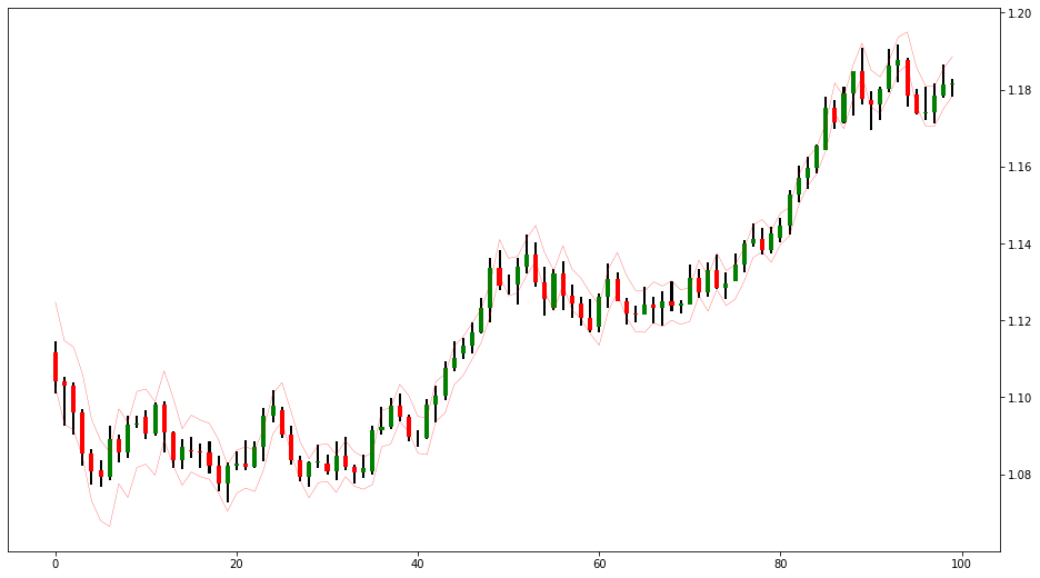

EURUSD daily momentum channel bands

欧元兑美元每日动能通道带

接下来做什么？ (What to do next?)

Well to be honest, if i would be making money using this strategy, i wouldn’t share it here with you (no offense). I wouldn’t even sell it. However, you can use your own imagination and add some strategies on this. You can thank me later if you decide to use this code and make money. I will send you my IBAN later :)

老实说，如果我要使用这种策略来赚钱，我不会在这里与您分享(无罪)。 我什至不卖。 但是，您可以发挥自己的想象力，并为此添加一些策略。 如果您决定使用此代码并赚钱，稍后可以感谢我。 稍后我将把您的IBAN发送给您：)

Disclaimer

免责声明

I’m not a professional financial advisor. This article and codes, shared for educational purposes only and not financial advice. You are responsible your own losses or wins.

我不是专业的财务顾问。 本文和代码仅用于教育目的，不用于财务建议。 您应对自己的损失或胜利负责。

The whole code of this article can be found on this repository:

可以在此存储库中找到本文的完整代码：

Ah also; remember to follow me on the following social channels:

也啊 记得在以下社交渠道关注我：

MediumTwitterTradingViewYouTube!

中级 Twitter TradingViewYouTube ！

Until next time; stay safe, trade safe!!!

直到下一次; 保持安全，交易安全！！！

Atilla Yurtseven

阿蒂拉·尤尔特斯文(Atilla Yurtseven)

翻译自: https://medium.com/swlh/trading-with-momentum-channels-in-python-f58a0f3ebd37

动量策略 python