可视化深度学习_深度学习中的准确性可视化第1部分

最新推荐文章于 2023-08-04 14:02:09 发布

weixin_26720761

最新推荐文章于 2023-08-04 14:02:09 发布

阅读量506

点赞数

文章标签：可视化深度学习机器学习人工智能 python

原文链接：https://towardsdatascience.com/accuracy-visualisation-in-deep-learning-part-1-b42d32b07913

版权

可视化深度学习

内部AI (Inside AI)

“One look is worth a thousand words.”

“一个表情值一千字。”

We all want to train the deep learning models in the most optimum way to increase even the last two decimal of the prediction accuracy. We have so many parameters to tweak in the deep learning model starting from the optimiser and its parameters, activation function, number of layers/filters etc. that finding the right combinations of all these parameters is like finding a needle in the haystack.

我们都希望以最优化的方式训练深度学习模型，以增加预测精度的最后两位。从优化器及其参数，激活函数，层/过滤器数量等开始，我们有很多参数需要调整，以至于在深度学习模型中进行调整，以至于找到所有这些参数的正确组合就像在大海捞针中找到一根针。

Fortunately, we can leverage hyperparameters to tune the performance and accuracy of the model, but we need to have a broad sense of the parameter combination to try and test.

幸运的是，我们可以利用超参数来调整模型的性能和准确性，但是我们需要对参数组合有广泛的了解才能尝试和测试。

Tensor board is one of the most powerful inbuilt tool available to visualise individual model’s performance based on different metrics and also for comparison among different models. It can guide in ascertaining the ballpark parameter combinations which we can further try with hyperparameter tuning.

Tensor板是可用的最强大的内置工具之一，可基于不同的指标可视化单个模型的性能，并用于不同模型之间的比较。它可以指导确定棒球参数组合，我们可以通过超参数调整进一步尝试这些组合。

In this article, I will discuss the deep learning model visualisation with a combination of optimisers and activation function for simple regression. It will enable us to learn how we can discard unsuitable combinations quickly and focus our performance tuning efforts on a few potential parameters.

在本文中，我将讨论优化器和激活函数相结合的深度学习模型可视化，以实现简单的回归。这将使我们能够学习如何快速丢弃不合适的组合，并将性能调整工作集中在一些潜在参数上。

Step 1: We will use the Scikit learn make_regression method to generate a random dataset for regression testing and train_test_split to divide the datasets into training and testing set.

步骤1：我们将使用Scikit学习 make_regression方法生成用于回归测试的随机数据集，并使用train_test_split将数据集分为训练和测试集。

from sklearn.datasets import make_regression
from sklearn.model_selection import train_test_split

Step 2: In the code below, we have imported the Tensor Board and deep learning Keras package. We will use Keras for modelling and Tensor Board for visualisation.

第2步： 在下面的代码中，我们导入了Tensor Board和深度学习Keras软件包。我们将使用Keras进行建模，并使用Tensor Board进行可视化。

from tensorflow.keras.callbacks import TensorBoard
from keras.models import Sequential
from keras.layers import Dense

Step 3: In this article, we will work with “adam” and “RMSprop” optimiser, and GlorotUniform” and “normal” weight initializer. We have mentioned these in a list and will call the combination in sequence for training the model.

步骤3：在本文中，我们将使用“ adam”和“ RMSprop”优化器，以及GlorotUniform”和“ normal”重量初始化器。我们已经在列表中提到了这些，并将按顺序调用组合以训练模型。

optimizers=["adam","RMSprop"] #Optimisers
initializers=["GlorotUniform","normal"] # Activation function

Step 5: In the below code, we have nested FOR loop to train the deep learning model with different combinations of optimisers and weight initialiser, and record the result for analysis in Tensor board.

步骤5：在下面的代码中，我们嵌套了FOR循环，以使用优化器和权重初始化器的不同组合来训练深度学习模型，并将结果记录在Tensor板上进行分析。

Each model is named with weight initialiser and optimiser name to identify each model’s result and graph.

每个模型都用权重初始化程序和优化程序名称命名，以标识每个模型的结果和图形。

As the main objective of this article is to learn the visualisation of deep learning model results, hence we will work with a very simple model with one input, hidden and output layer.

本文的主要目的是学习深度学习模型结果的可视化，因此我们将使用一个具有一个输入，隐藏和输出层的非常简单的模型。

We will use mean square error as a loss function for all the model and measure the mean absolute percentage error. If you do not know these statistical metrics, then I will suggest referring Wikipedia for detail explanation.

我们将均方误差用作所有模型的损失函数，并测量平均绝对百分比误差。如果您不了解这些统计指标，那么我建议您参考Wikipedia进行详细说明。

Step 6: We can view the results and analyse after the code is executed. We need to open the command prompt in windows or terminal in mac to start the Tensor Board. Navigate to the folder directory in where logs are saved via command prompt/terminal and then type the below command.

步骤6：执行代码后，我们可以查看结果并进行分析。我们需要在Windows或Mac的终端中打开命令提示符以启动Tensor Board。通过命令提示符/终端导航到保存日志的文件夹目录，然后键入以下命令。

tensorboard --logdir=logs/

It will instantiate the tensor board and will show the address which we need to type in the browser to view the results.

它将实例化张量板，并显示我们需要在浏览器中键入以查看结果的地址。

In the current example, we can access the Tensor board by typing http://localhost:6006/ in the browser.

在当前示例中，我们可以通过在浏览器中输入http：// localhost：6006 /来访问Tensor板。

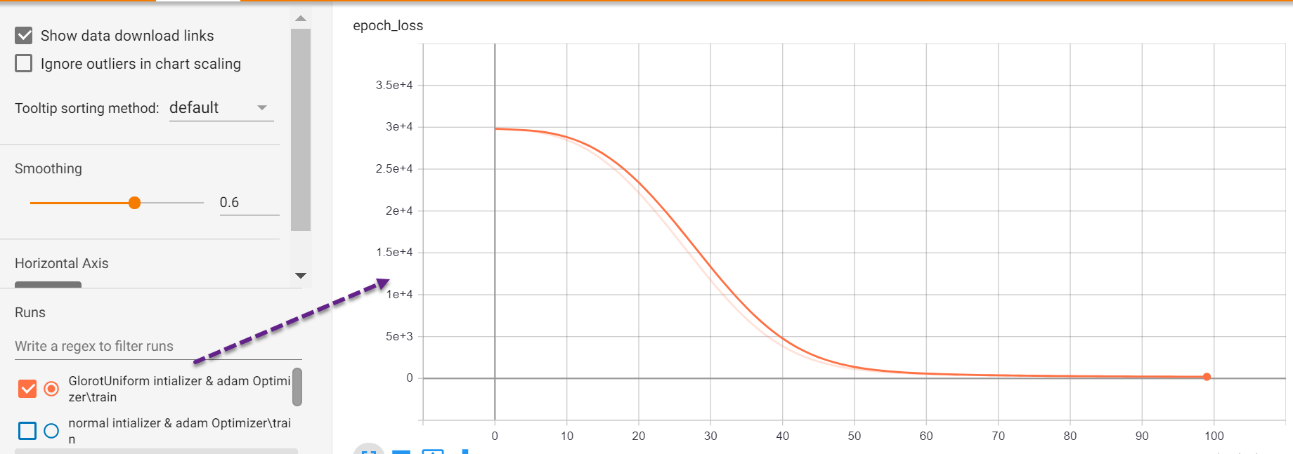
In one consolidated graph, we can view the change in the mean square error as the number of iterations progresses for a different combination of optimizers and weight initializers.

在一个合并的图中，对于优化器和权重初始化器的不同组合，随着迭代次数的进行，我们可以查看均方误差的变化。

It indicates the optimizers and weight initializers which are unsuitable for the current datasets and modelling. In the current example, the mean squared loss is decreasing way slower for “RMSprop” and “normal” optimiser combination than other combinations. Based on this knowledge from the visualisation, we can focus our energy in fine-tuning the remaining combinations and save time by not tweaking the combination which is not performing well on a broad level.

它指示不适合当前数据集和建模的优化器和权重初始化器。在当前示例中，“ RMSprop”和“ normal”优化器组合的均方损失下降速度比其他组合慢。基于从可视化中获得的知识，我们可以将精力集中在微调剩余的组合上，并通过不调整在广泛水平上效果不佳的组合来节省时间。

In the same way, we can view the change in mean absolute percentage error for different combinations as the number of iterations progresses.

同样，我们可以查看随着迭代次数的增加，不同组合的平均绝对百分比误差的变化。

We can also use filters to view the graphs of one or more combination of the models.

我们还可以使用过滤器来查看一个或多个模型组合的图形。

It is important to give meaningful names to the model as it helps to put the filter correctly and avoid confusion during the analysis. In the current example, the combination of weight initializer and optimiser is the name of the model.

给模型起有意义的名字很重要，因为它有助于正确放置过滤器并避免在分析过程中造成混淆。在当前示例中，权重初始化程序和优化程序的组合是模型的名称。

We can also download the graphs, and loss function data SVG and CSV format respectively. Loss function data in CSV format enables us to perform advanced analysis quickly with excel.

我们还可以分别下载图形和损失函数数据SVG和CSV格式。 CSV格式的损失函数数据使我们能够使用excel快速执行高级分析。

Besides visualising the result in terms of epochs progression, we can also view the relative performance of the model with a single click of a mouse.

除了根据历时进展可视化结果外，我们还可以通过单击鼠标来查看模型的相对性能。

In this article, we have learnt the basics of the tensor board and seen a few visualisation options available to grasp the finer details about different models in an instant. We also saw the way we can use the tensor board visualisation to focus on fine-tuning potential models. In the next article, we will see a few advanced visualisations for deep learning models.

在本文中，我们了解了张量板的基础知识，并看到了一些可视化选项可用于立即掌握有关不同模型的更详细信息。我们还看到了可以使用张量板可视化来专注于微调潜在模型的方法。在下一篇文章中，我们将看到深度学习模型的一些高级可视化效果。

If you would like to learn Exploratory data analysis (EDA) with visualisation then read by article 5 Advanced Visualisation for Exploratory data analysis (EDA)

如果您想学习可视化的探索性数据分析(EDA)，请阅读第5条探索性数据分析(EDA)的高级可视化。

If you are a big fan of pandas like me then you will find the article 5 Powerful Visualisation with Pandas for Data Preprocessing interesting to read and learn.

如果您是像我这样的大熊猫爱好者，那么您会发现阅读和学习文章5强大的可视化熊猫与熊猫进行数据预处理。