python bs期权模型_使用python第二部分建立股票期权评估模型

python bs期权模型

In Part I, I went over how we could use the yahoo_fin module to access stock and option pricing data, and we generated payoffs under different scenarios.

在第一部分中 ，我介绍了如何使用yahoo_fin模块访问股票和期权定价数据，并在不同情况下产生了收益。

What we aim to do now is figure out an expected payoff.

我们现在的目标是找出预期的收益。

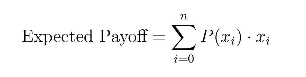
In our case, the expected payoff of an option contract is the sum of each payoff times the probability of reaching that payoff.

在我们的案例中，期权合约的预期收益是每个收益的总和乘以达到该收益的可能性。

For example, in part I we showed the various payoffs for an AT&T option under scenarios ranging from a -50% price drop to a +50% price gain:

例如，在第一部分中，我们展示了在价格下跌-50％到价格上涨+ 50％的情况下，AT＆T期权的各种收益：

If we now generate the probability of each price % change, we can then compute the sum of the payoff and probability vectors to gain our expected payoff.

如果现在生成每个价格％变动的概率，则可以计算收益和概率向量的总和，以获得期望的收益。

生成价格变化的概率分布 (Generating a Probability Distribution of Price Changes)

Stocks can move up and down. Predicting the price of a stock in a week is theoretically impossible (without inside information). Yet, we can have some idea about the relative probabilities of how a stock might move.

股票可以上下波动。 理论上不可能在一周内预测股票价格(没有内部信息)。 但是，我们可以对股票如何移动的相对概率有所了解。

For example, if Procter & Gamble’s stock is trading at $135, and rarely ever fluctuates below $110 or above $150, then it is very unlikely that it will be $160 in a week.

例如，如果宝洁公司的股价为135美元，并且很少在110美元以下或150美元以上波动，那么一周内160美元的可能性就很小。

While we might not be able to use a stock’s historical price data to predict its price, we can use it to generate a distribution of potential price changes based on past experience.

虽然我们可能无法使用股票的历史价格数据来预测其价格，但是我们可以根据过去的经验使用它来生成潜在价格变化的分布。

#Importing required modules:import pandas as pd
import numpy as np
import matplotlib.pyplot as plt
import random
import datetimedef delta_dist(ticker, duration, sample_size):
   stock = get_data(ticker).close
   dates = list(stock.index)
   duration = int(duration)
   sample_size = int(sample_size)
   deltas = []for s in range(sample_size):try:
         x = random.randint(0, (sample_size - 1))
         start = stock[x]
         stop = stock[x + duration]
         difference_percent = (stop - start)/start
         deltas.append(difference_percent) except:
         pass   return deltas

In the code above, delta_dist() will take in a stock ticker, duration (time period to estimate price change over), and sample_size.

在上面的代码中， delta_dist()将接收一个股票报价器，持续时间( 估计价格变化的时间段 )和sample_size。

Suppose we ran delta_dist( ‘AAPL’ , 14, 1000). This function would choose 1000 random days to pull price info on Apple’s stock. It will then find the difference between the stock price of that day and 14 days ahead for each day sampled. I use a try and except within the loop in case one of the days sampled happened to be within the last 14 days (in which case it could not calculate the difference, since 14 days ahead of it would be in the future).

假设我们运行了delta_dist( 'AAPL' , 14, 1000) 。 此功能将随机选择1000天以获取苹果股票的价格信息。 然后，它将针对该采样日找到当天和未来14天的股价之间的差额。 我try了try ， except在循环中except ，以防万一采样的天恰好在最近的14天之内(在这种情况下，它无法计算出差异，因为将来可能是14天)。

As shown above, we want to find probabilities over each 1% interval. Therefore, we want to bin the results that delta_dist() returns:

如上所示，我们希望找到每个1％间隔的概率。 因此，我们要对delta_dist()返回的结果进行delta_dist() ：

def binned(diffs):
   bins = [] for bin in range(101):    #needs to be 101 to count -50% and +50%
      begin = (bin - 50)*0.01def between_bins(k):return (k <= begin + .01) and (k > begin)
      count = list(filter(between_bins, diffs))
      amount = len(count)/len(diffs)  #amount is percent of total
      bins.append(amount)return(bins)

Using binned(), we can count up the frequency of times a price change falls within each 1% interval.

使用binned() ，我们可以计算出价格变化落入每个1％间隔内的次数。

Let’s use Apple as an example:

让我们以Apple为例：

#EXAMPLE : SAMPLE SIZE 200changes = delta_dist('AAPL', 14, 200)
binned_changes = binned(changes)
x_axis = np.arange(-50, 51, 1)plt.bar(x_axis, binned_changes)
plt.xlabel('Stock Price % Change')
plt.ylabel('Probability')
plt.title('AAPL: Probability Distribution- 14 day price change(Sample Size=200)');
plt.savefig('AAPL_prices.png', dpi = 800)

This will generate the probability distribution of a 14 day price change using a sample of 200 random days in which Apple was on the market:

这将使用苹果在市场上随机出现的200天样本生成14天价格变化的概率分布：

Here is what it looks like when we adjust the sample size to 9000 days:

将样本量调整为9000天后，结果如下所示：

And here is what it looks like when we look at average prices over 3 years, rather than two weeks:

这是当我们查看三年而不是两周的平ASP格时的样子：

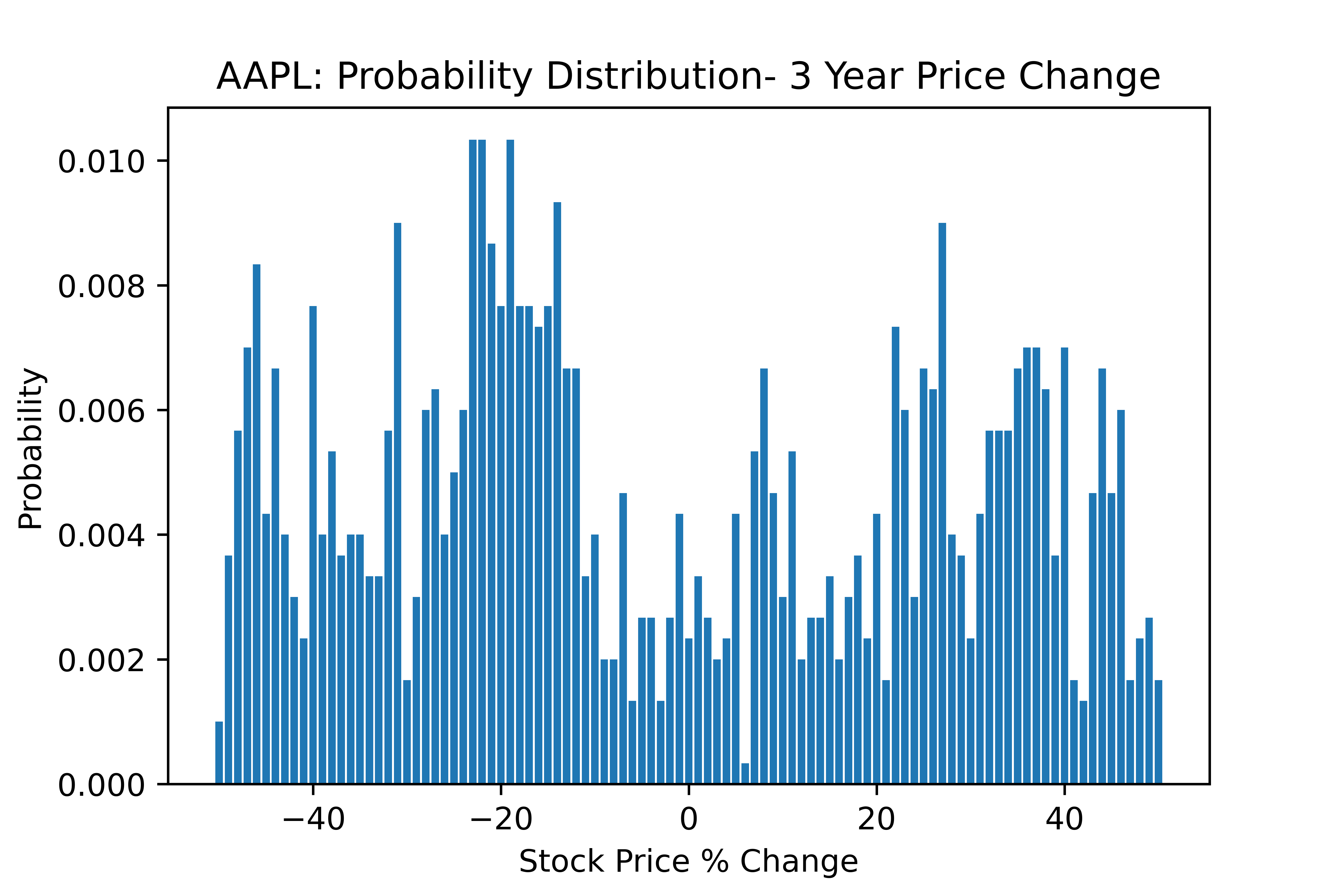
As you might expect, the probability of larger price swings is much greater over longer time periods.

如您所料，在更长的时间内，更大的价格波动可能性更大。

将价格变动概率应用于我们的期权数据集 (Applying Price Change Probabilities to our Options Dataset)

The options_df dataset from Part I contains options expiring on September 18th. Therefore, it would be useful to know the amount of time between that expiration date and today.

第一部分中的options_df数据集包含9月18日到期的选项。 因此，了解该到期日期与今天之间的时间量将很有用。

To do this, we use the datetime module and subtract today’s date from the expiration. We then create a dictionary containing each ticker as a key along with a list containing the probability distribution from [-50% , +50%].

为此，我们使用datetime模块，并从到期datetime减去今天的日期。 然后，我们创建一个包含每个股票行情作为键的字典，以及一个包含[-50％，+ 50％]概率分布的列表。

#Generate time lapse between today and expiration of options contract:timedate_until_exp = datetime.strptime(expiration, '%B %d, %Y') - datetime.today()#convert day number to integer:time_until_exp = int(timedate_until_exp.days)scenario_tickers = list(set(options_df.Ticker))
number_of_tickers = len(scenario_tickers)
simulations = 2000#dict_of_stuff will contain each ticker key corresponding to the 101 values of its distribution of price changes [-50%, 50%]dict_of_probs = dict()for stock in scenario_tickers:     
   changes = delta_dist(stock, time_until_exp, simulations)
   distribution_list = binned(changes)  
   dict_of_probs.update({stock : distribution_list}) 

To test that our code worked, let’s see a random example taken from dict_of_probs.

为了测试我们的代码是否有效，让我们看一下从dict_of_probs中获取的随机示例。

#Verify it works with examplex_axis = np.arange(-50, 51, 1)
example = random.randint(0, number_of_tickers - 1)
plt.bar(x_axis, dict_of_probs[scenario_tickers[example]])
plt.xlabel('Stock Price % Change')
plt.ylabel('Probability')
plt.title(str(time_until_exp) + " day average % price change for " + str(scenario_tickers[example]))
plt.savefig('price_example.png', dpi = 800)

Success! At this point, we have both a straightforward method to generate our payoff distribution and a dictionary containing the average % price change distribution for each stock ticker.

成功！ 在这一点上，我们既有一种简单的方法来生成我们的收益分布，又有一个字典，其中包含每个股票行情记录器的平ASP格变动百分比。

计算预期收益 (Calculating Expected Payoffs)

Photo by Sharon McCutcheon on Unsplash

Sharon McCutcheon在 Unsplash上 拍摄的照片

Suppose that the price of Apple stock has a 10% probability of increasing by 1% in two weeks. Let’s say you see an options contract with a 2-week expiration that generates $20 in profit if Apple is up 1%. Therefore, the expected payoff of that contract on the [0 , 1%] interval would be $20 * 0.1 = $2.

假设苹果股票的价格在两周内有10％的可能性上涨1％。 假设您看到一份为期2周的期权合约，如果苹果股价上涨1％，该合约便产生20美元的利润。 因此，该合约在[0，1％]区间上的预期收益为$ 20 * 0.1 = $ 2。

If you did this for every 1% interval of that contract (which we will assume is from -50% to +50%), and sum up the results, then you would have the overall expected payoff of the contract.

如果您以该合同的每1％间隔(假设为-50％到+ 50％)进行此操作，然后对结果进行汇总，那么您将获得合同的总体预期收益。

This is what we will do for every contract within our options_df.

这是我们将对options_df每份合同执行的操作。

#Generating expected payoffsx_axis = np.arange(-50, 51, 1)
ExpectedPay = []for i in range(len(options_df)):
   payoffs = []
   ticker = options_df.iloc[i].Tickerfor p in range(len(x_axis)):
      percent = (p - 50)*0.01
      payoff = price_percent_payoff(percent, options_df.iloc[i])
      payoffs.append(payoff)
   probs = dict_of_probs[ticker]
   expected_value = sum( np.array(probs) * np.array(payoffs) )
   ExpectedPay.append(expected_value)options_df['ExpectedPay'] = ExpectedPay

At this point, we now have our expected payoff for each options contract. Let’s see how the payoffs look:

至此，我们现在有了每个期权合约的预期收益。 让我们看看收益如何：

plt.hist(ExpectedPay, bins = 40, range=[-2000, 2000])
plt.xlabel('Total Expected Gain/Loss of Contract in $')
plt.ylabel('Frequency')
plt.title("Frequency of Expected Gains and Losses");
plt.savefig('payoffs.png', dpi = 800)

You will notice that most options have an expected payoff around $0. This makes sense since the contract is hedging risk among buyer and seller.

您会注意到，大多数期权的预期收益约为$ 0。 这是有道理的，因为合同正在对冲买卖双方之间的风险。

Remember that an option is a zero-sum game. If I purchase a call option (providing me the right to buy at the strike price), then someone else has purchased a put option (they sell me the stock at that strike price if I exercise it).

请记住，一个选项是零和游戏。 如果我购买了看涨期权 (向我提供了按行使价购买的权利)，那么其他人已经购买了看跌期权 (如果我行使行使价，他们会以该行使价向我出售股票)。

Therefore, an efficient market would bring the expected value of most contracts to zero (as buyers and sellers are not going to get ripped off).

因此，有效的市场将使大多数合同的预期价值为零(因为买卖双方不会被剥夺)。

Still, we can notice that there are contracts on the right tail that could possibly provide profitable investments.

不过，我们可以注意到，在右边的合同可能会提供有利可图的投资。

In practice, this dataset can provide some insight into options worth looking more into. The payoffs calculated should not be used to make investment decisions, and those looking to trade options should do further research into why those expected payoffs are as high/low as they are.

实际上，该数据集可以提供一些值得深入研究的选项的见解。 计算出的收益不应该用于做出投资决策，而那些寻求交易期权的收益应该做进一步的研究，以了解那些预期收益为何如此之高/低。

One other significant point not yet discussed is that many of these ‘profitable’ contracts might appear so due to low liquidity. That is, the Volume and Open Interest could both be very low, suggesting no one is actually trading based on what the Bid-Ask spread that we use.

尚未讨论的另一个重要点是，由于流动性低，许多“获利”合同可能会出现。 也就是说，交易Volume和未Open Interest Volume都可能很低，这表明没有人根据我们使用的买入/卖出价差实际进行交易。

With that being said, I plan to further tweak this model to provide more insight into valuing options with different expirations and to account for low liquidity issues.

话虽如此，我计划进一步调整此模型，以提供更多洞察力来评估具有不同到期日的期权并解决流动性低的问题。

翻译自: https://medium.com/@jacoblingerr/building-a-stock-option-valuation-model-with-python-part-ii-c93262d41d0b

python bs期权模型