LSTM实践多变量时间序列预测

本文是

第一部分数据处理：

数据下载：开源能源系统数据

from pandas import read_csv
from datetime import datetime
from matplotlib import pyplot
# load data

dataset = read_csv('raw1.csv',  parse_dates = [0], index_col=0)
dataset.drop('CY_load_entsoe_transparency', axis=1, inplace=True)
dataset.drop('CY_wind_onshore_generation_actual', axis=1, inplace=True)
# manually specify column names
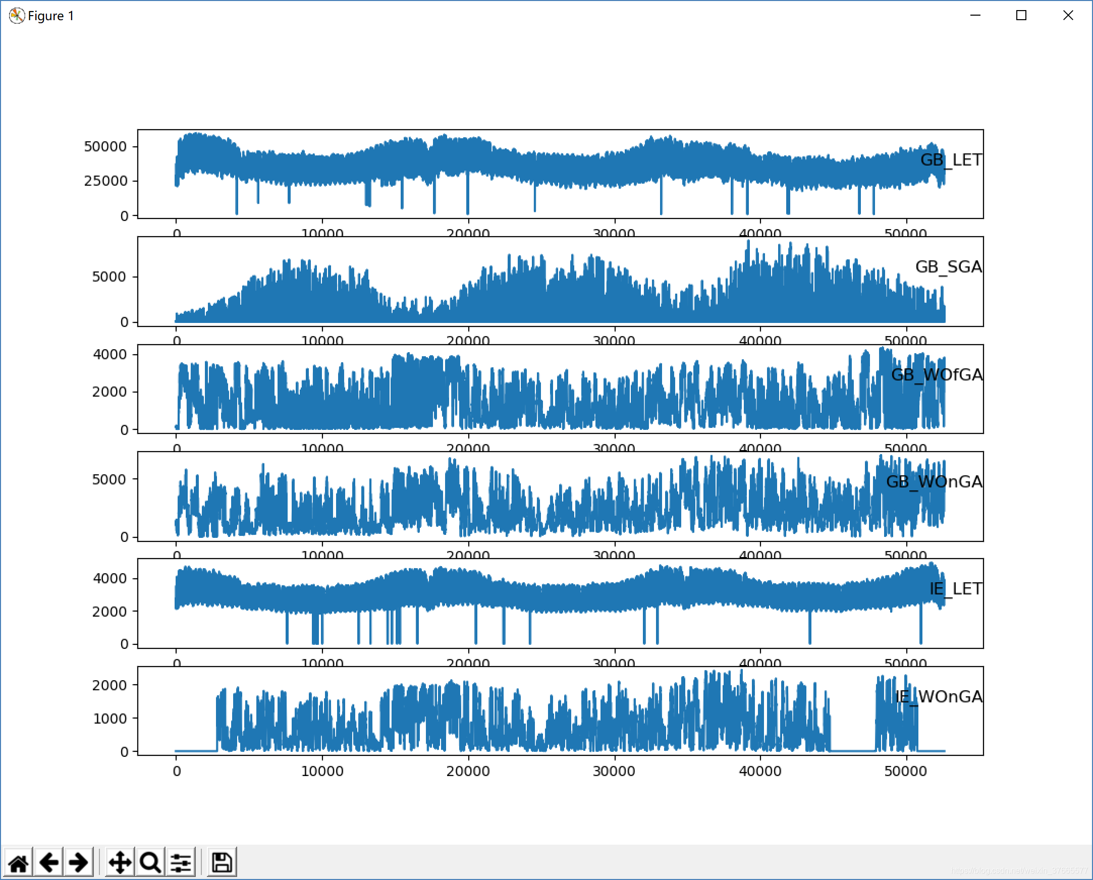
dataset.columns = ['LET', 'SGA', 'WOfGA', 'WOnGA']
dataset.index.name = 'date'
# mark all NA values with 0
dataset['LET'].fillna(0, inplace=True)
dataset['SGA'].fillna(0, inplace=True)
dataset['WOfGA'].fillna(0, inplace=True)
dataset['WOnGA'].fillna(0, inplace=True)
# drop some rows
dataset = dataset[456:35544]#取[456:35544]两年的数据
# summarize first 5 rows
print(dataset.head(5))
# save to file
dataset.to_csv('use.csv')
# load dataset
dataset = read_csv('use.csv', header=0, index_col=0)
values = dataset.values
print(values)
groups = [0, 1, 2, 3]
i = 1
# plot each column
pyplot.figure()
for group in groups:
	pyplot.subplot(len(groups), 1, i)
	pyplot.plot(values[456:1000, group])
	pyplot.title(dataset.columns[group], y=0.5, loc='right')
	i += 1
pyplot.show()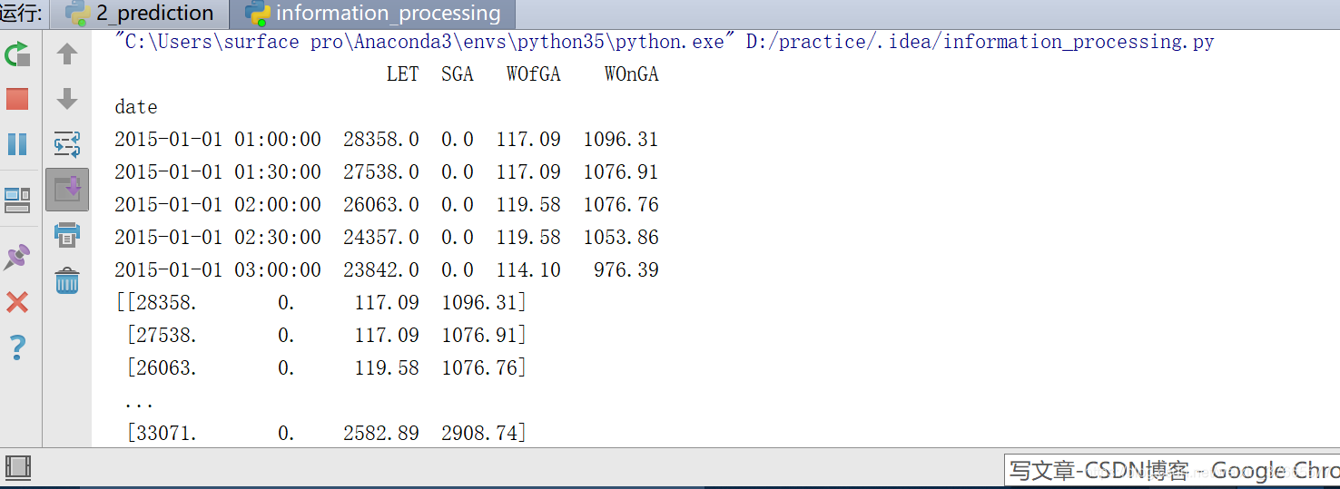

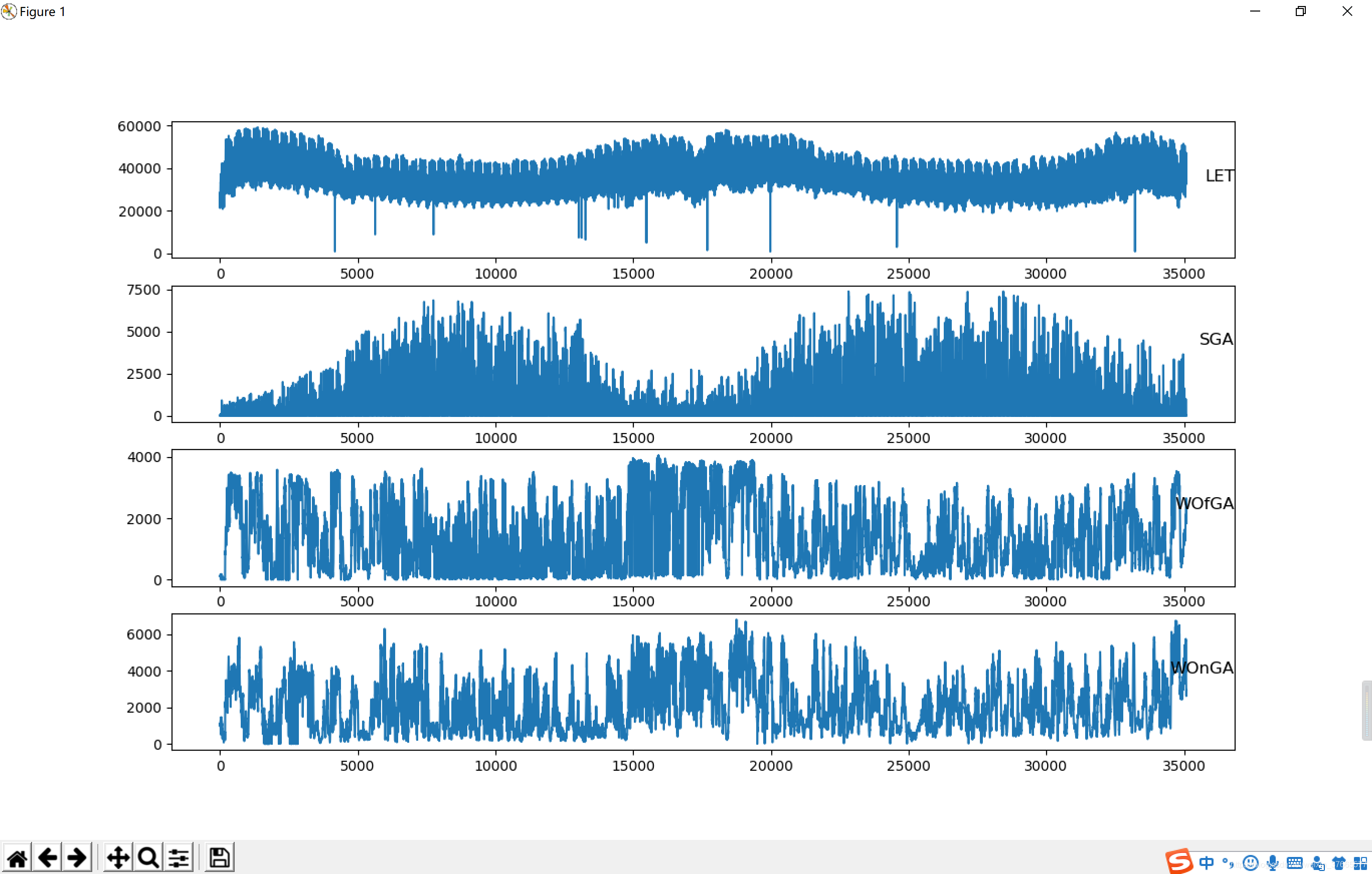
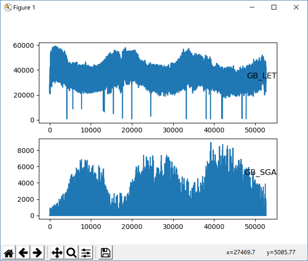
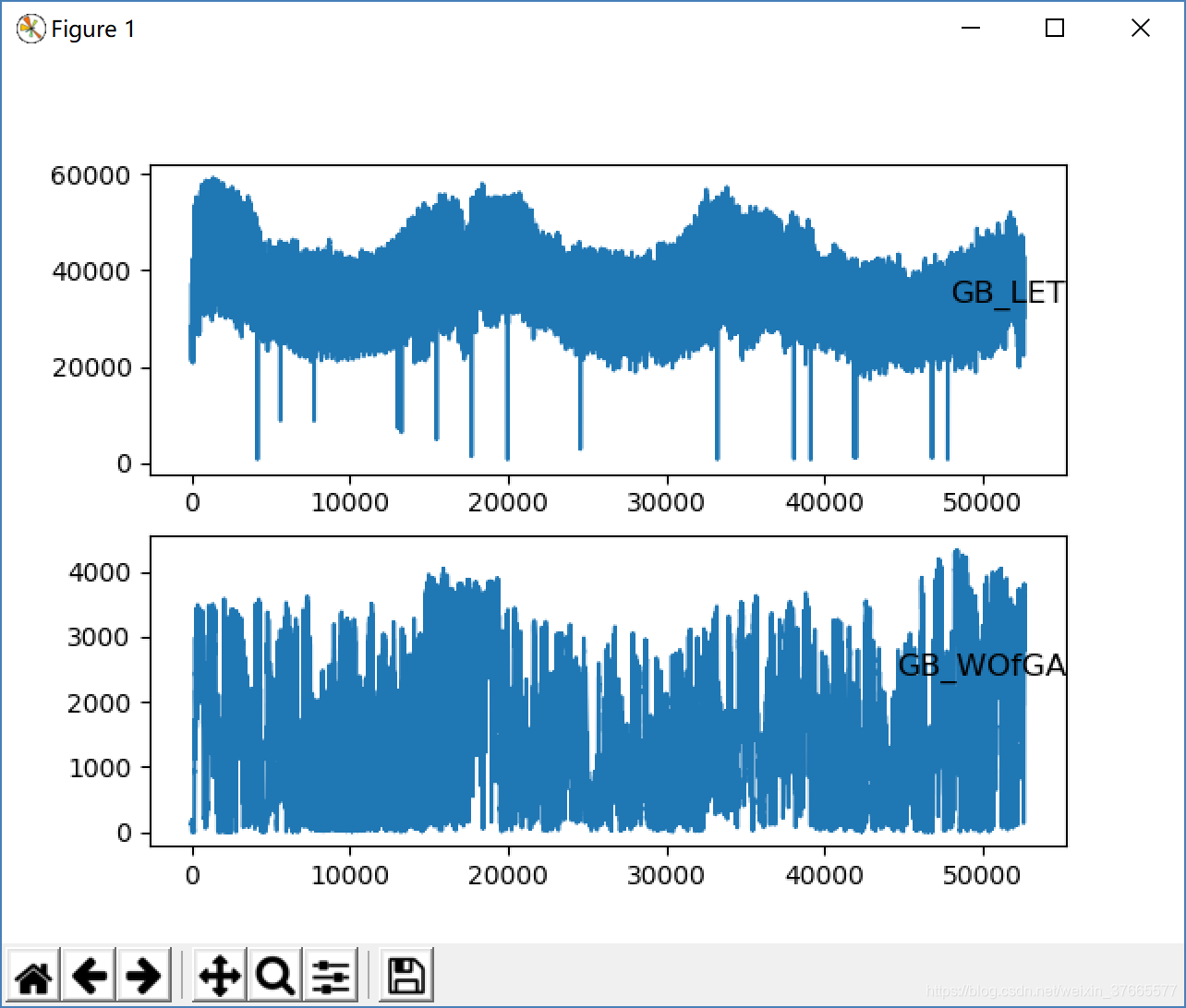
画出两年的趋势

可以看出有些数据很明显是错误的

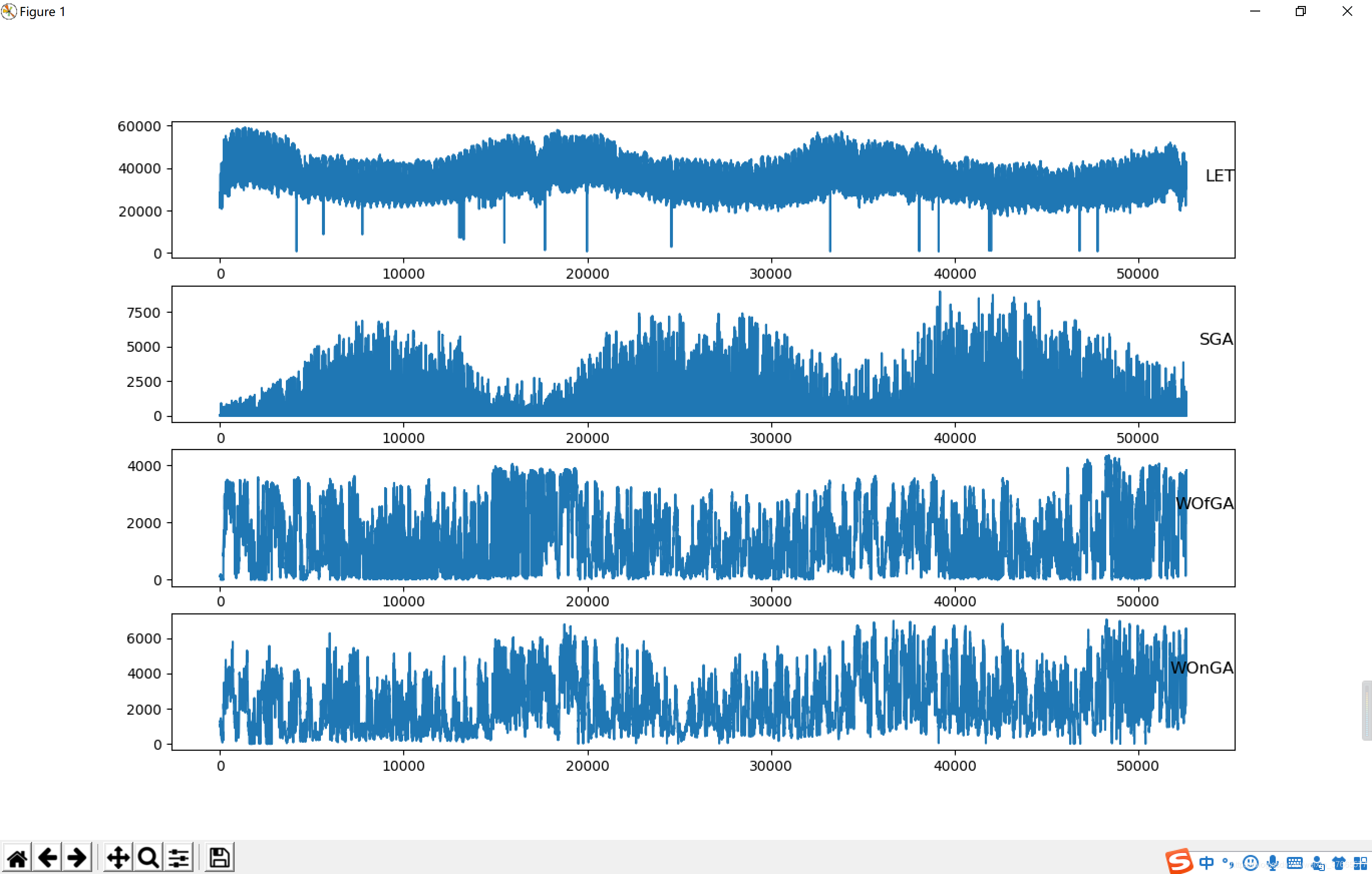
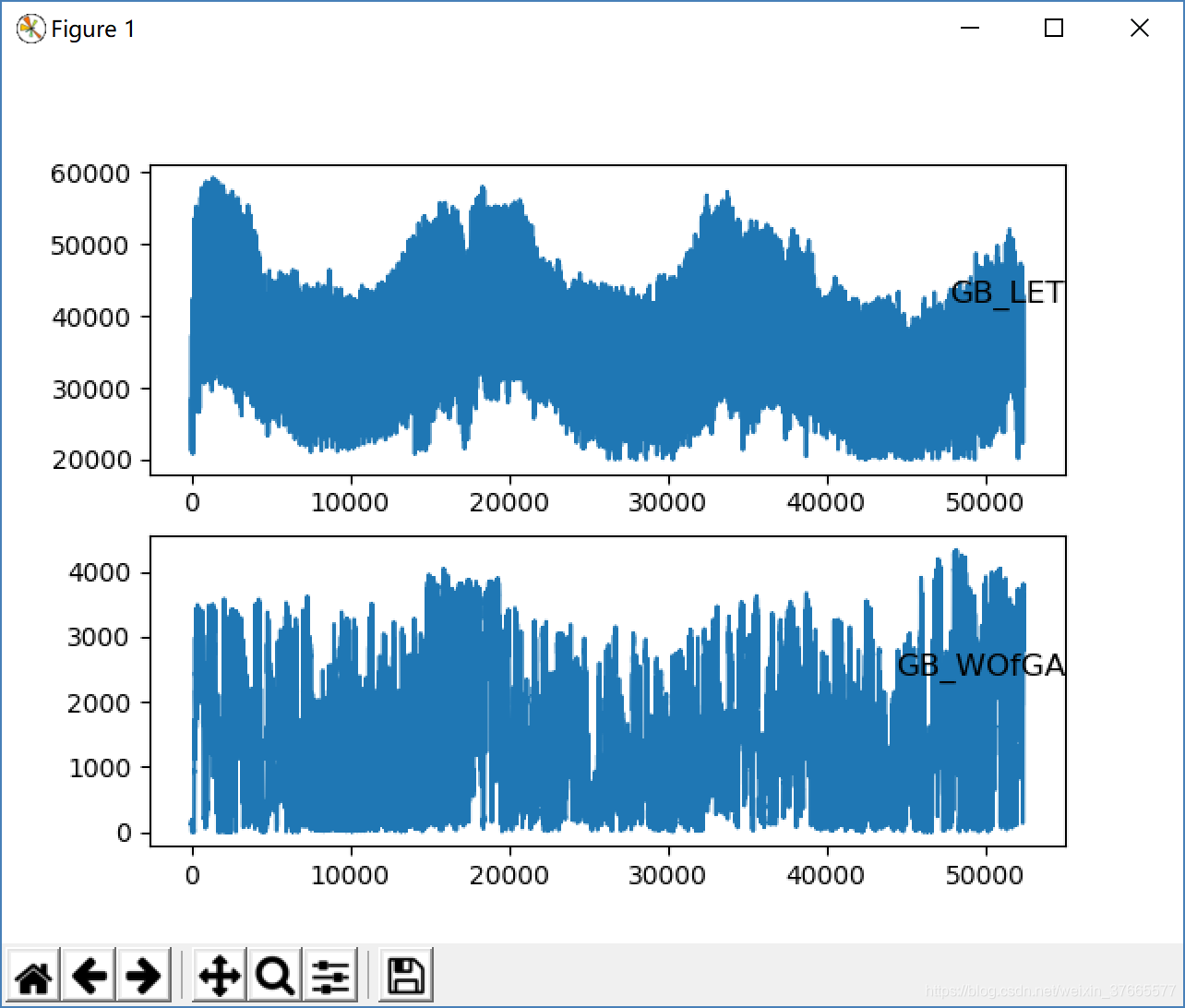
这个数据有两年半年完整的数据把15-17年的画出来，趋势更明显

这里应该加上数据处理

 

 

接下来就是搭建网络和预测

from math import sqrt
from numpy import concatenate
from matplotlib import pyplot
from pandas import read_csv
from pandas import DataFrame
from pandas import concat
from sklearn.preprocessing import MinMaxScaler
from sklearn.preprocessing import LabelEncoder
from sklearn.metrics import mean_squared_error
from keras.models import Sequential
from keras.models import load_model
from keras.layers import Dense
from keras.layers import LSTM


# convert series to supervised learning
def series_to_supervised(data, n_in=1, n_out=1, dropnan=True):
	n_vars = 1 if type(data) is list else data.shape[1]
	df = DataFrame(data)
	cols, names = list(), list()
	# input sequence (t-n, ... t-1)
	for i in range(n_in, 0, -1):
		cols.append(df.shift(i))
		names += [('var%d(t-%d)' % (j+1, i)) for j in range(n_vars)]
	# forecast sequence (t, t+1, ... t+n)
	for i in range(0, n_out):
		cols.append(df.shift(-i))
		if i == 0:
			names += [('var%d(t)' % (j+1)) for j in range(n_vars)]
		else:
			names += [('var%d(t+%d)' % (j+1, i)) for j in range(n_vars)]
	# put it all together
	agg = concat(cols, axis=1)#返回新的连接数组
	agg.columns = names#The column labels of the DataFrame.
	# drop rows with NaN values
	if dropnan:
		agg.dropna(inplace=True)
	return agg

# load dataset
dataset = read_csv('use3.csv', header=0, index_col=0)
values = dataset.values
# integer encode direction:
encoder = LabelEncoder()
#values[:] = encoder.fit_transform(values[:])#将DataFrame中的每一行ID标签分别转换成连续编号
# ensure all data is float
values = values.astype('float32')
# normalize features
scaler = MinMaxScaler(feature_range=(0, 1))
scaled = scaler.fit_transform(values)
# frame as supervised learning
reframed = series_to_supervised(scaled, 1, 1)
# drop columns we don't want to predict
reframed.drop(reframed.columns[[4,5,7]], axis=1, inplace=True)
print(reframed.head())

# split into train and test sets
values = reframed.values
n_train_hours = 365 * 48
train = values[:n_train_hours, :]
test = values[n_train_hours:, :]
# split into input and outputs
train_X, train_y = train[:, :-1], train[:, -1]
test_X, test_y = test[:, :-1], test[:, -1]
# reshape input to be 3D [samples, timesteps, features]
train_X = train_X.reshape((train_X.shape[0], 1, train_X.shape[1]))
test_X = test_X.reshape((test_X.shape[0], 1, test_X.shape[1]))
print(train_X.shape, train_y.shape, test_X.shape, test_y.shape)

# design network
model = Sequential()
model.add(LSTM(50,
			   input_shape=(train_X.shape[1], train_X.shape[2])
			   ))
model.add(Dense(1))
model.compile(loss='mae', optimizer='adam')
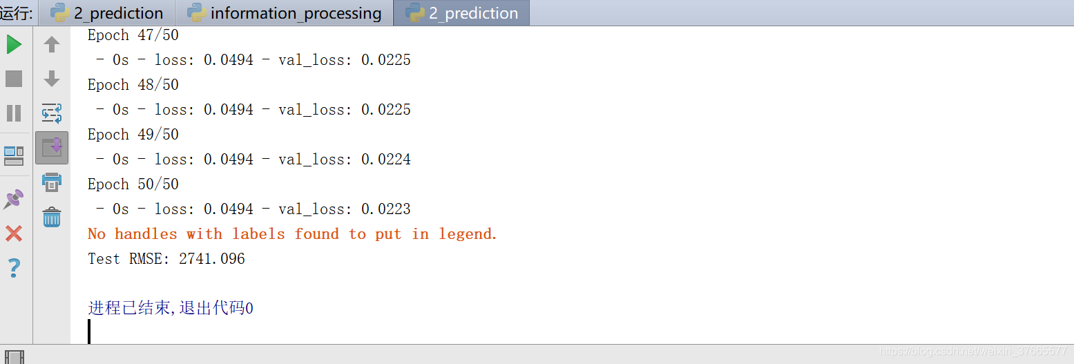
# fit network
history = model.fit(train_X, train_y, epochs=50, batch_size=120, validation_data=(test_X, test_y), verbose=2, shuffle=False)
'''# plot history
pyplot.plot(history.history['loss'], label='train')
pyplot.plot(history.history['val_loss'], label='test')
pyplot.legend()
pyplot.show()
'''
model.save('LSTM.h5')
# make a prediction
yhat = model.predict(test_X,96)
print(yhat[:5],yhat.shape)


print('prediction',yhat)
test_X = test_X.reshape((test_X.shape[0], test_X.shape[2]))
# invert scaling for forecast
inv_yhat = concatenate((yhat, test_X[:, 1:]), axis=1)
inv_yhat = scaler.inverse_transform(inv_yhat)
inv_yhat = inv_yhat[:,0]
# invert scaling for actual
test_y = test_y.reshape((len(test_y), 1))
inv_y = concatenate((test_y, test_X[:, 1:]), axis=1)
inv_y = scaler.inverse_transform(inv_y)
inv_y = inv_y[:,0]
# calculate RMSE
rmse = sqrt(mean_squared_error(inv_y, inv_yhat))
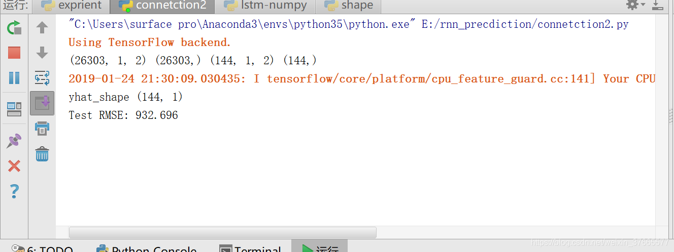
print('Test RMSE: %.3f' % rmse)

又发现两组数据，之前为了方便之间删除了，现在再加回来

 

这次把这个模型保存下来，下次预测前就不用训练了

model.save('LSTM.h5')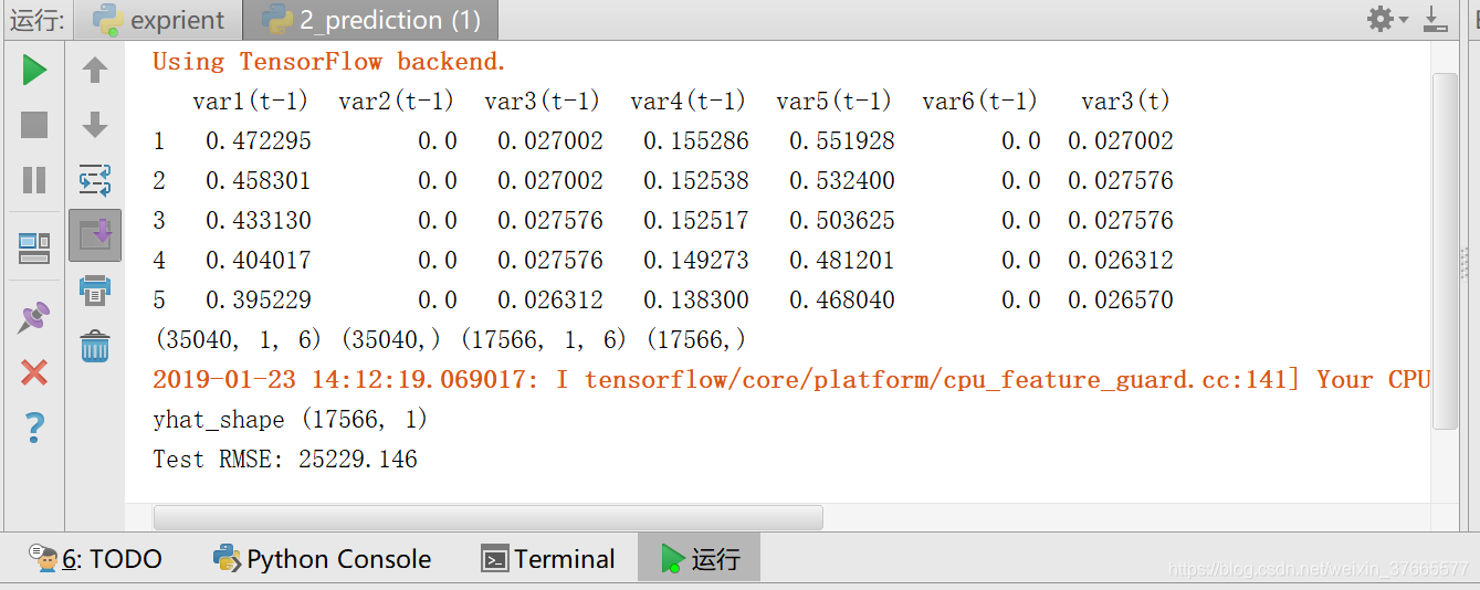

均方差：25229.146

均方根太大了

原因是这几个数据之间关联不大，没必要放在一起，从原始数据的图上看估计后三个应该和GB_LET有关

所以接下来只处理三者之一和GB_LET

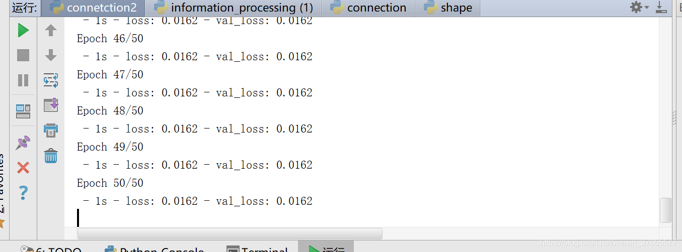
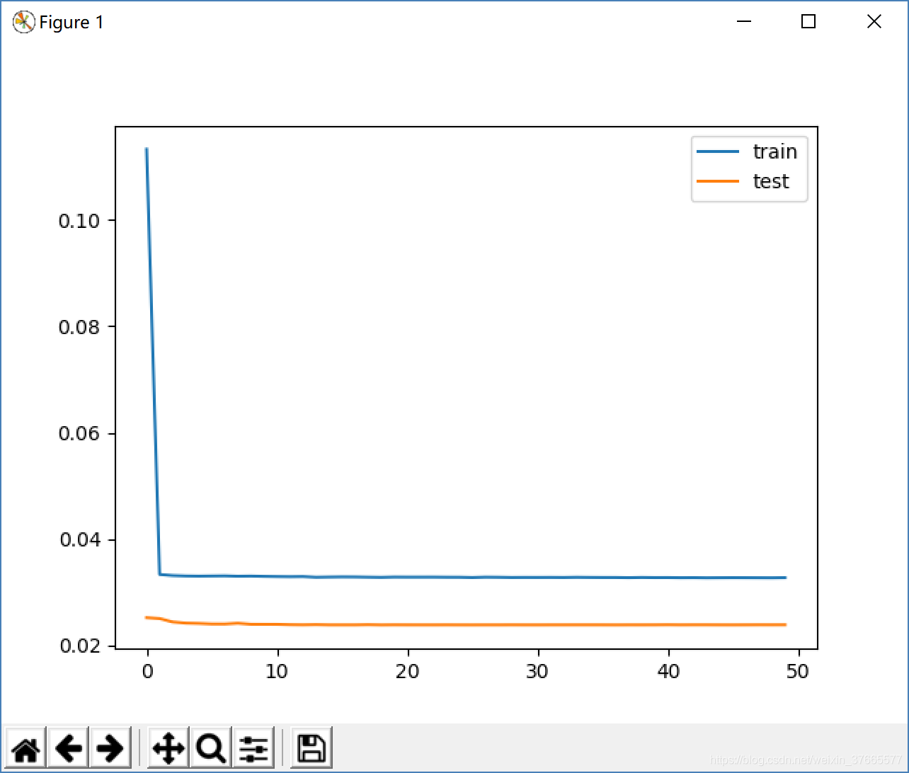
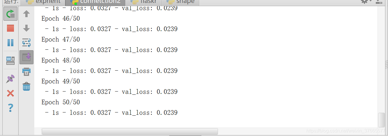
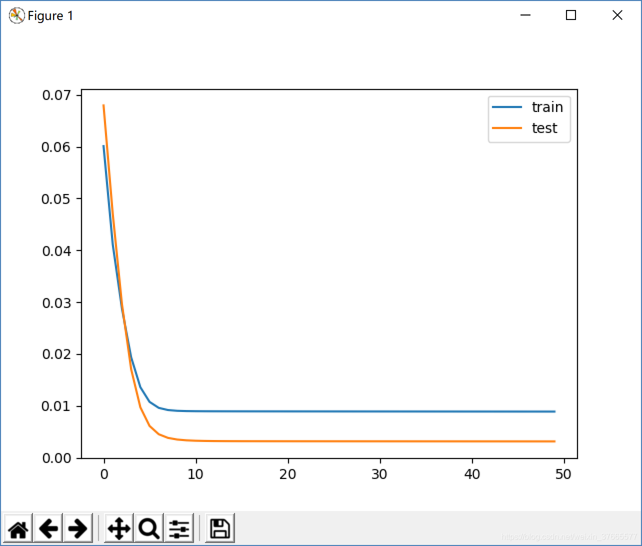
训练下来的训练集和测试集的loss比之前小很多

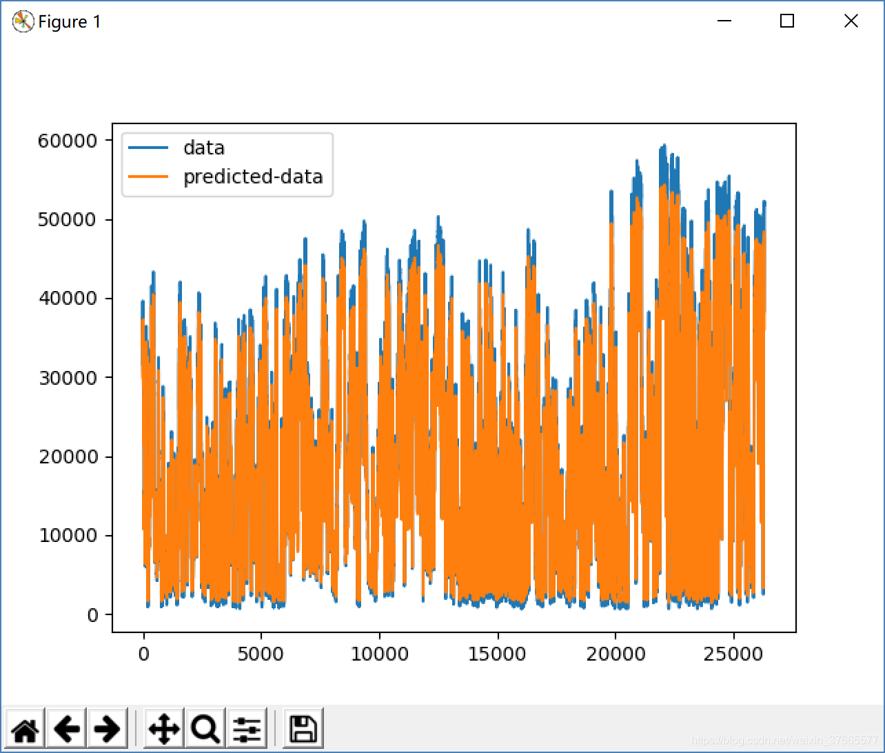
预测GB_LET

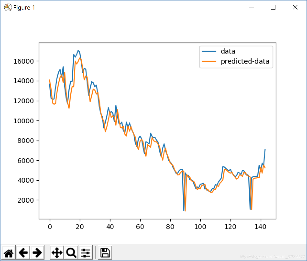
预测另一个GB_WOfGA

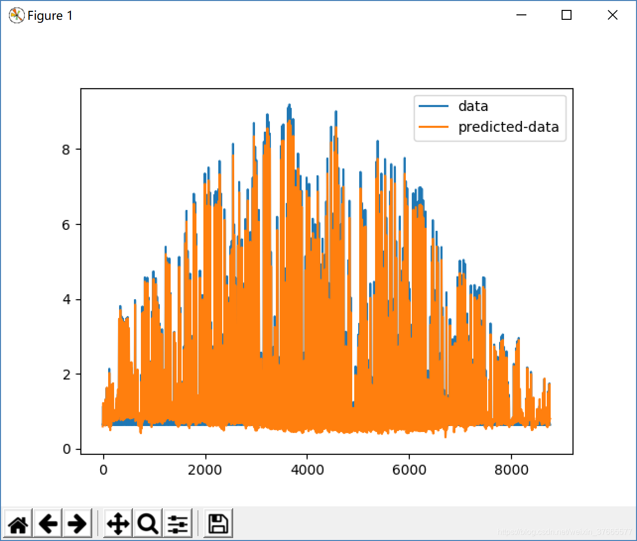
设置函数输出144个数据，实际和预测值如下：

sgd = optimizers.SGD(lr=0.0015, decay=1e-6, momentum=0.9, nesterov=True)
model.compile(loss='mean_squared_error', optimizer=sgd)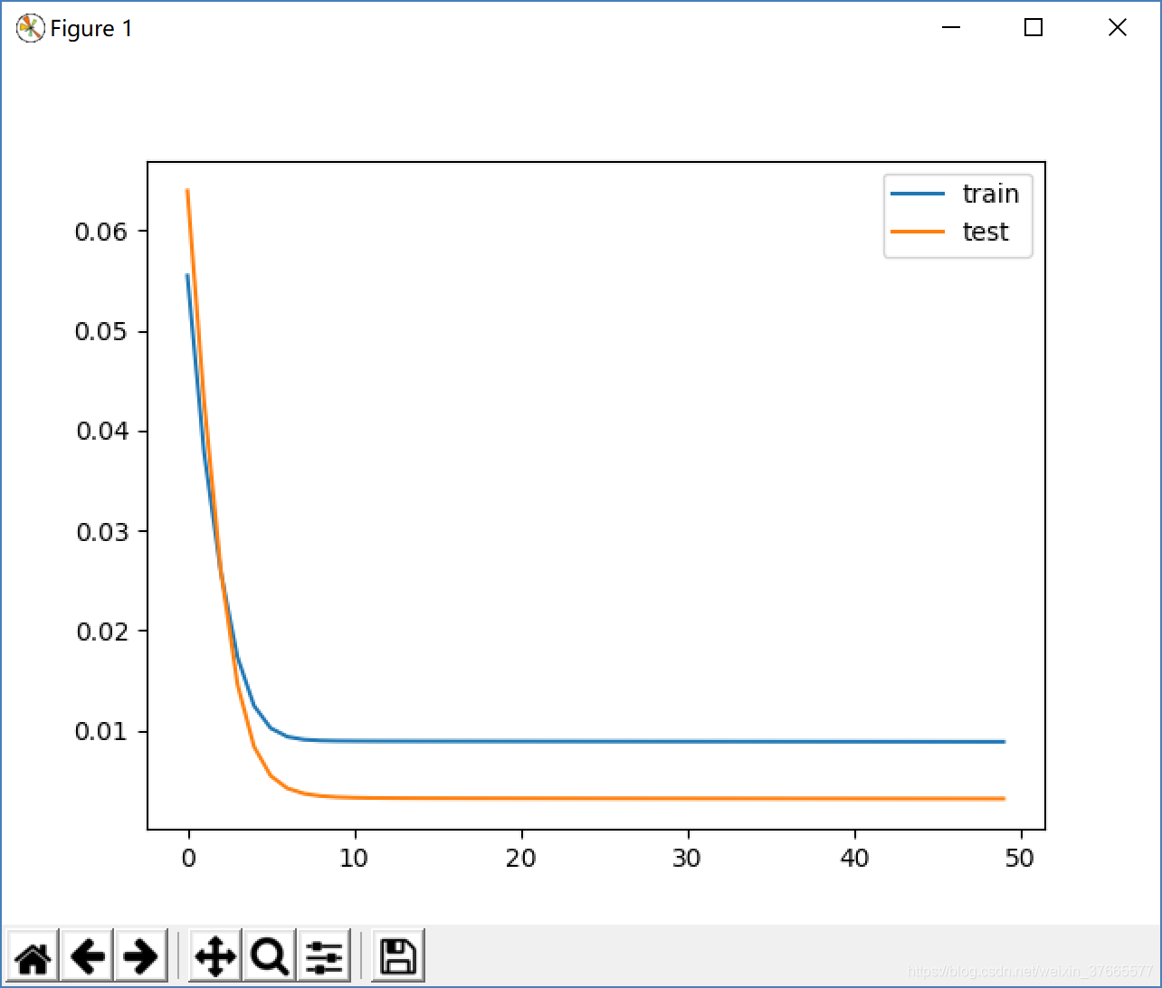

#去掉异常值
dataset.drop(dataset[(dataset["GB_LET"])<20000].index,inplace = True)

把这个模型保存下来命名为LSTM_without_outlier.h5

RMSE：3300.717

感觉这个误差变大好多。。。

再找些影响因素多的数据集来吧。

同一个网站里weather_data,取前四列来分析

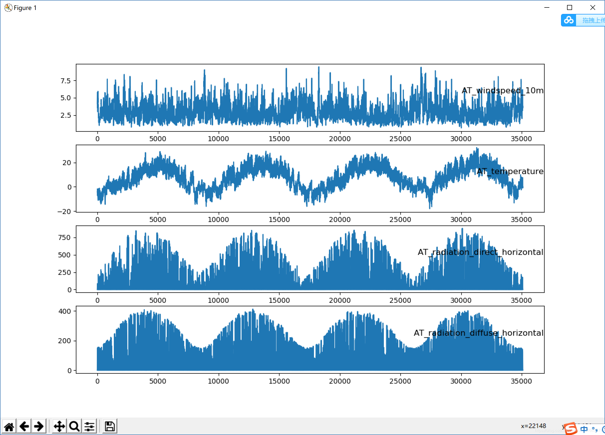
根据风速和温度预测辐射范围，首先预测radiation_direct_horizontal

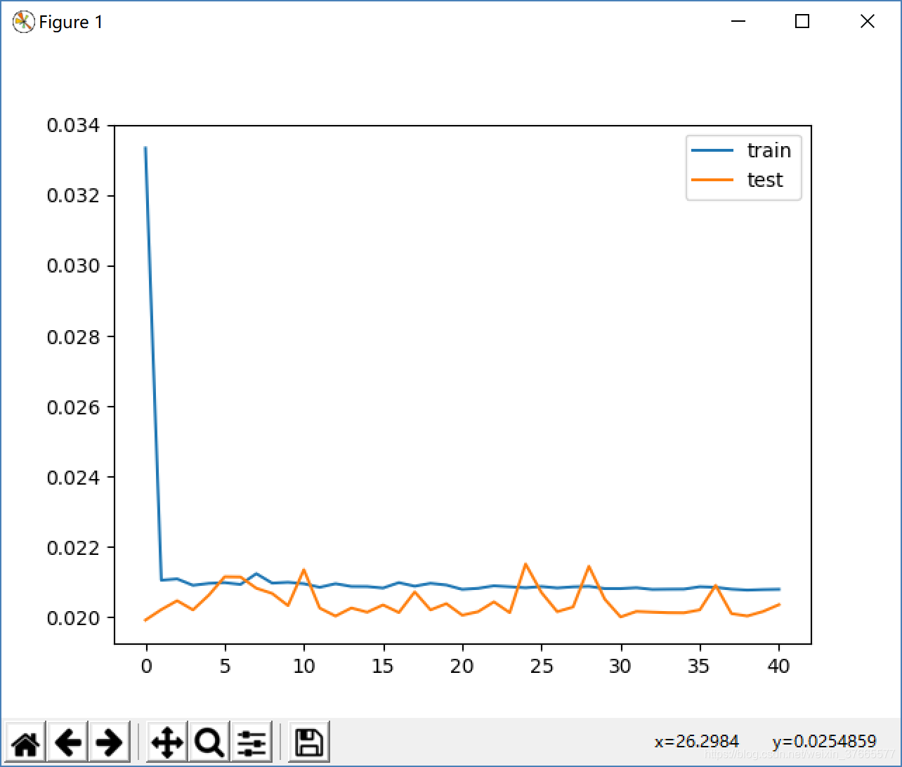
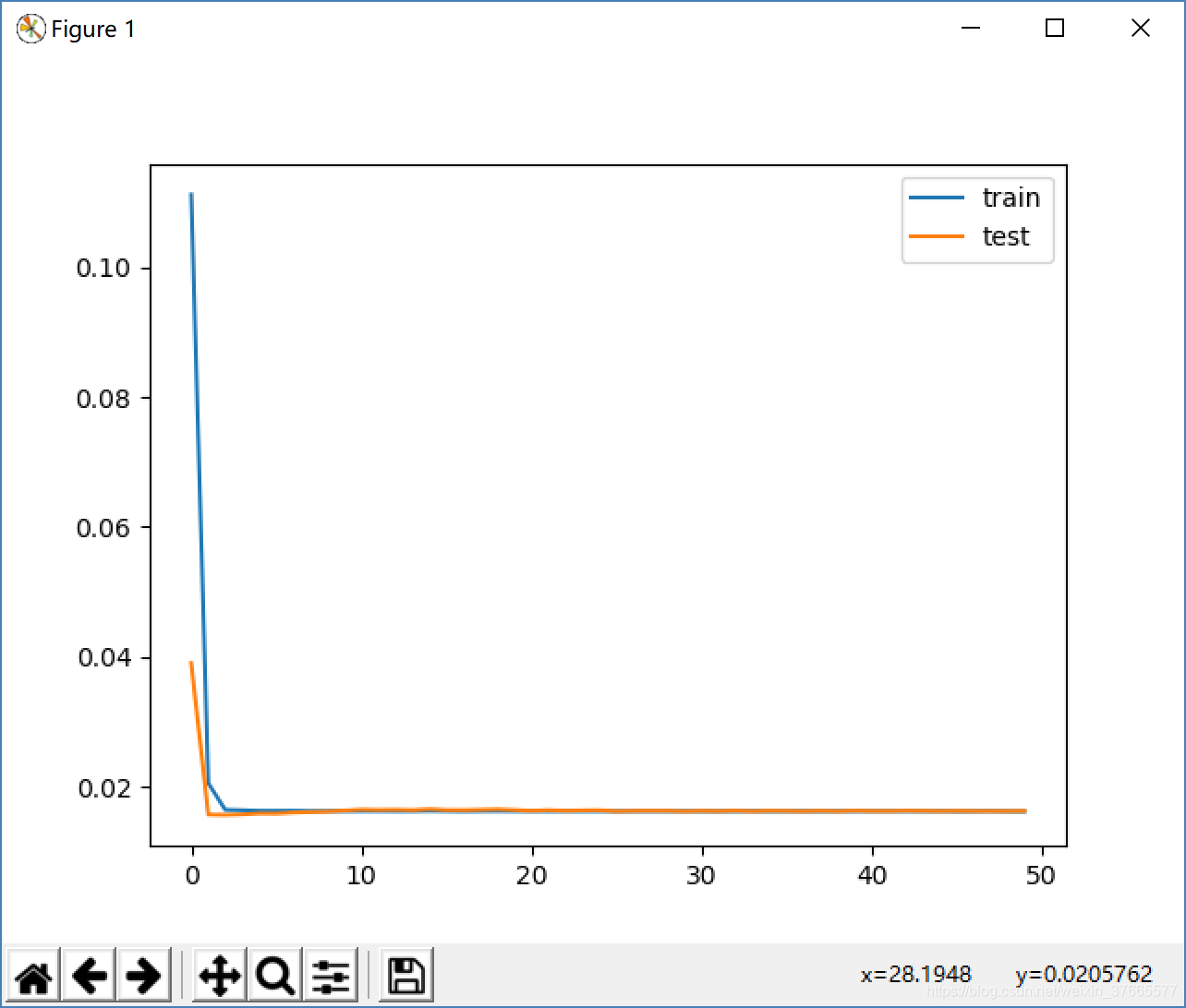
这个测试集的LOSS很不稳定

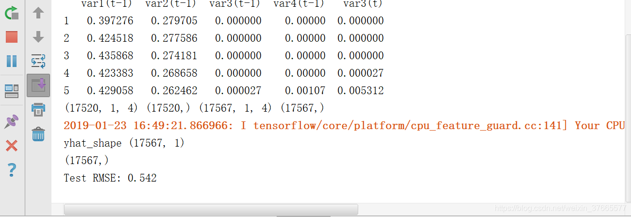
均方差：0.542

还是挺小的

 

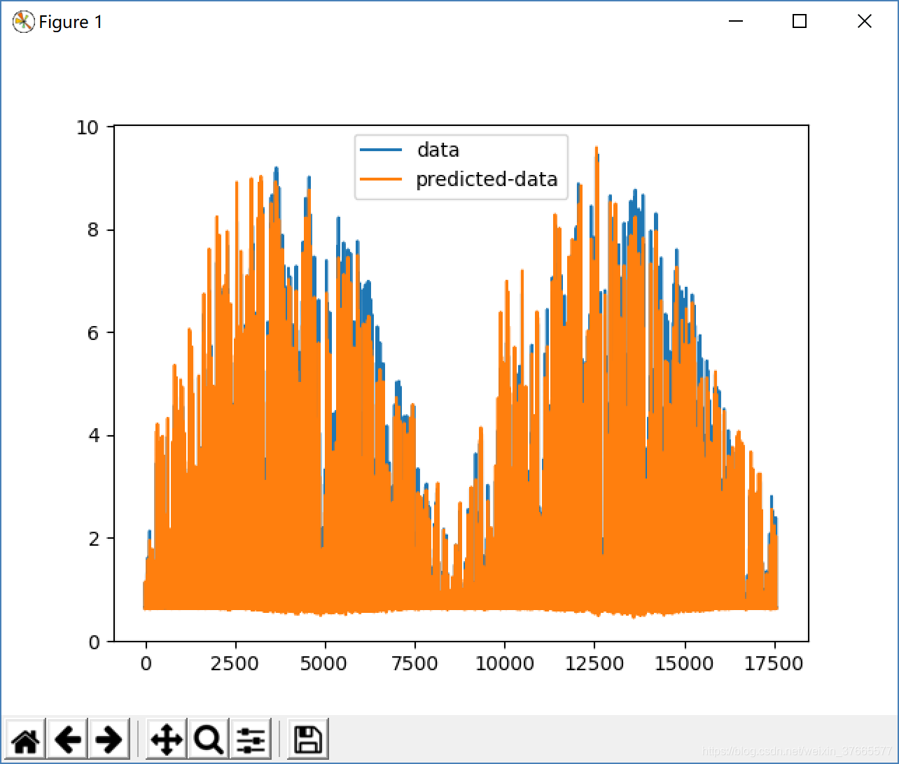
预测radiation_direct_horizontal

1.模型学习效果：

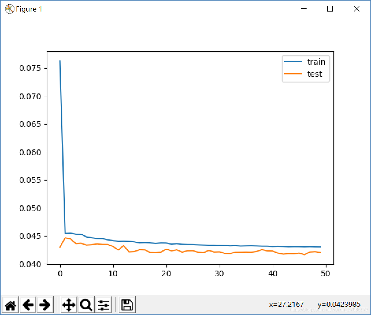
加入dropout后

dropout 用于模型在训练数据上损失函数较小，预测准确率较高；但是在测试数据上损失函数比较大，预测准确率较低。

优化之优化器学习率

之前使用优化器Adam，使用默认值

第二次改为学习率为0.01的梯度下降法

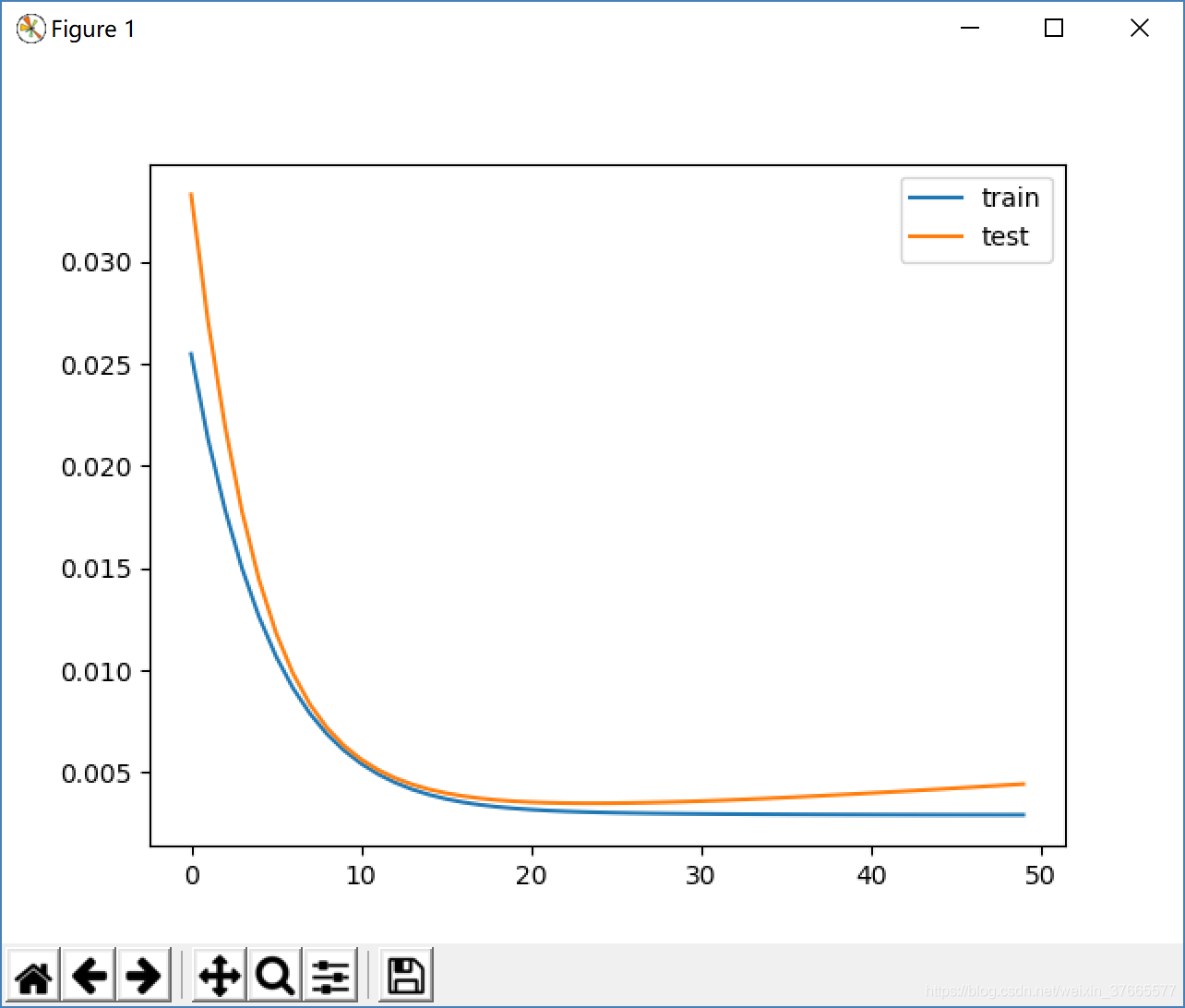
再多训练50个epoch

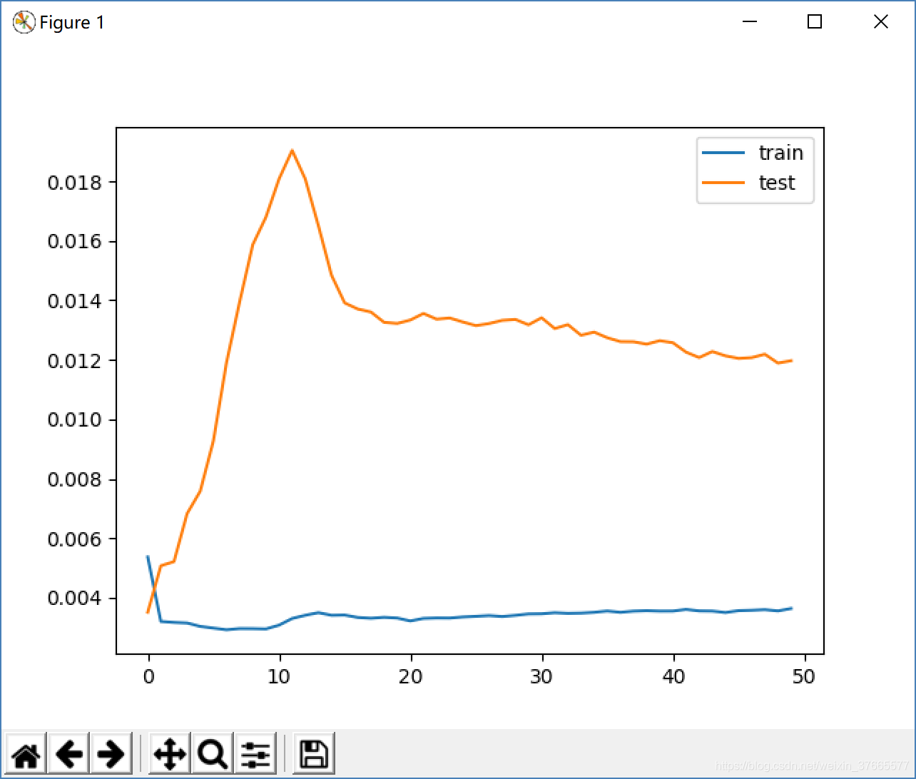
学习率下降了很多，大于20步后又变大了，看来数据出现过拟合

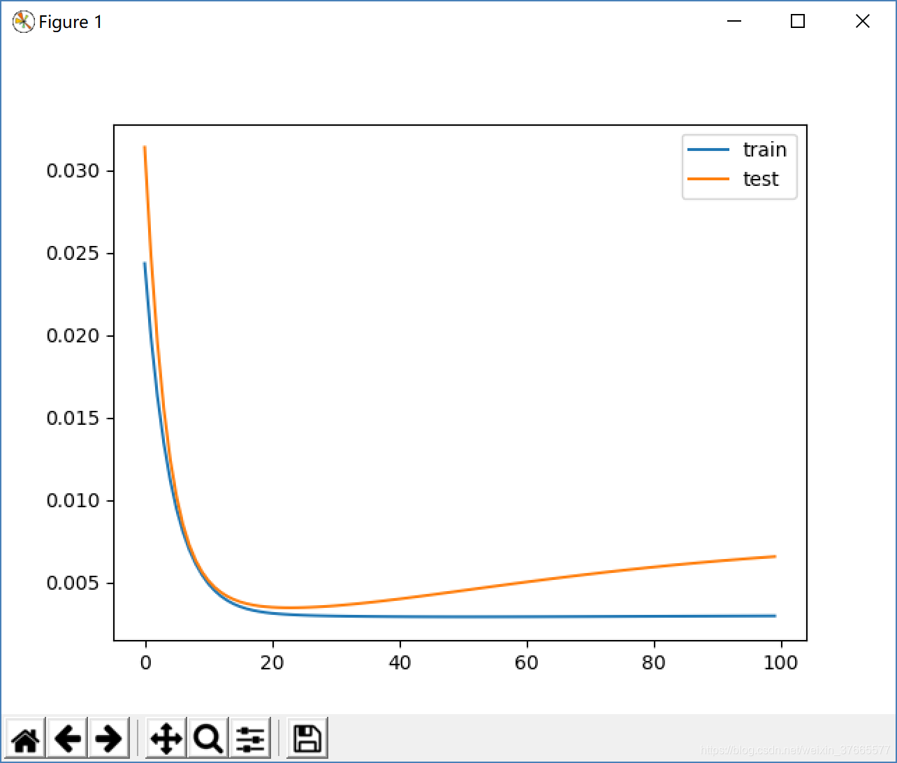
加入dropout(0.1)，调整学习率到0.009

使用adam优化器，设置学习率为0.009时数据明显过拟合了

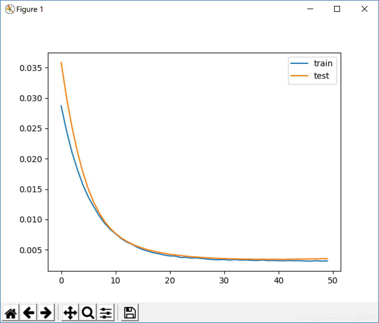
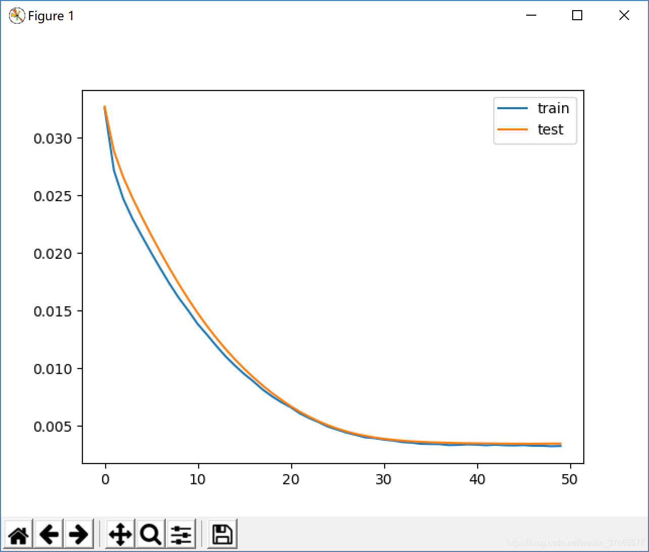
设置dropout为0.18，学习率为0.0001拟合的非常好，正好降低到0.0034之前几次训练mse的最低值，并且稳定了

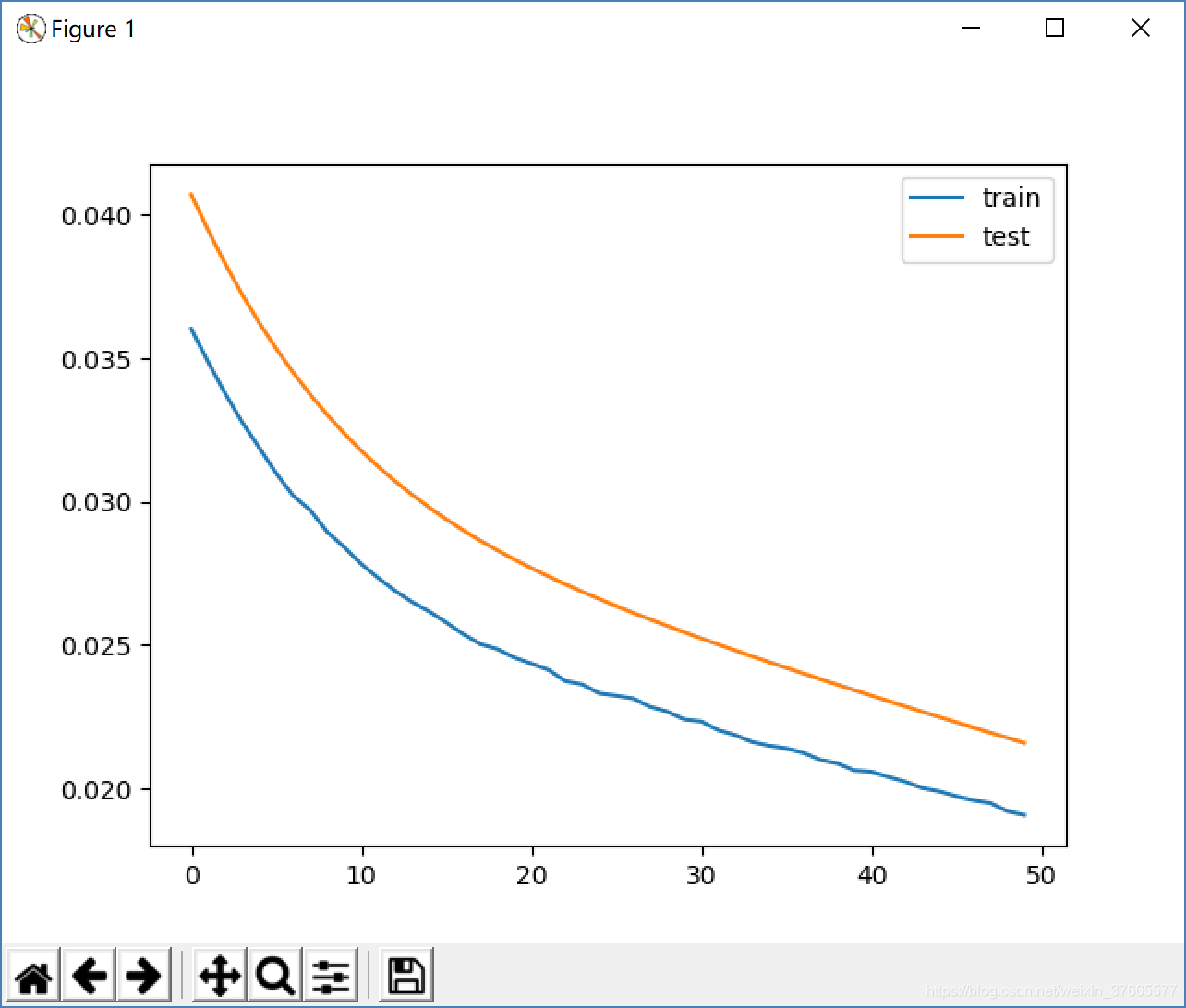
学习率为0.00001时，出现了过偏差

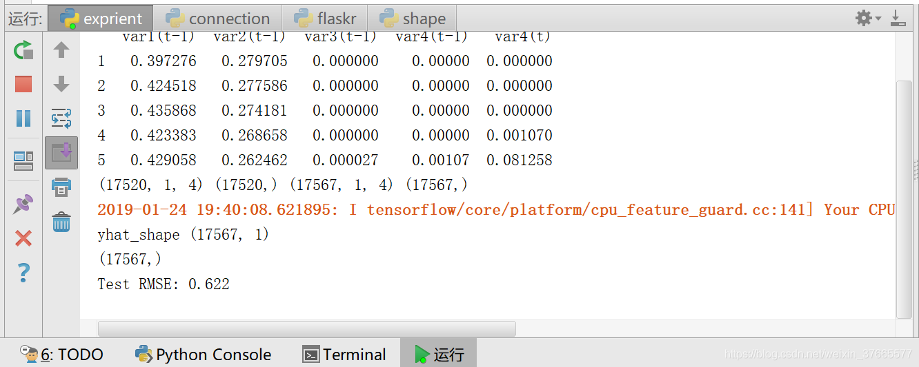
用之前的adm训练好的模型预测一个月的数据：

Test RMSE: 0.609

预测一年的数据，Test RMSE: 0.523

预测的优劣有几个因素决定：

1、样本集截取位置，应该输入整年的数据

2、数据之间的相关性

 

一些难点：

1. 如何将时间序列问题转化为监督学习问题

个人理解：与xs(t)也就是训练目标在DATAFRAME中相对应的应该ys(t+1)，即其预测的值同时刻的真实值