[opencv][python] 学习手册3：练习代码3

最新推荐文章于 2023-08-07 13:42:07 发布

飞天牛牛

最新推荐文章于 2023-08-07 13:42:07 发布

阅读量177

点赞数

分类专栏： opencv

本文链接：https://blog.csdn.net/weixin_37834269/article/details/111874144

版权

opencv 专栏收录该内容

33 篇文章 2 订阅

订阅专栏

[opencv][python] 学习手册3：练习代码3

56_Canny算法.py
57_双边滤波器.py
58_示例_霍夫直线.py
59_查找棋盘上的直线.py

文章目录

[opencv][python] 学习手册3：练习代码3

56_Canny算法.py

原理

Canny算法由John F.Canny于1986年开发，是很常用的边缘检测算法。

它是一种多阶段算法，内部过程共4个阶段：

噪声抑制（通过Gaussianblur高斯模糊降噪）:使用5x5高斯滤波器去除图像中的噪声
查找边缘的强度及方向（通过Sobel滤波器）
应用非最大信号抑制（Non-maximum Suppression）: 完成图像的全扫描以去除可能不构成边缘的任何不需要的像素
高低阈值分离出二值图像（Hysteresis Thresholding）

高（T2）低（T1）阈值比例：T2:T1 = 3:1 / 2:1

在这里插入图片描述

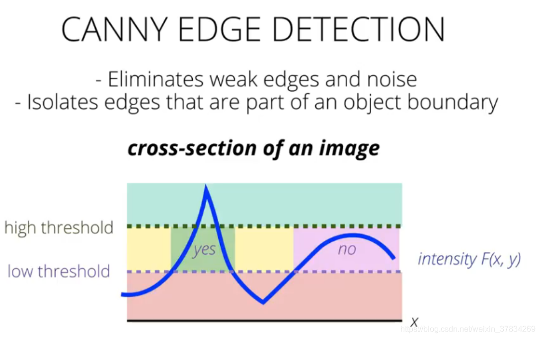
去掉大于高阈值以及低于低阈值的信息，保留他们之间的信息作为边缘，没有同时触及两个阈值的信息一并去掉。

代码

"""
Canny 算法
它是一种多阶段算法，内部过程共4个阶段：

1. 噪声抑制（通过Gaussianblur高斯模糊降噪）:使用5x5高斯滤波器去除图像中的噪声
2. 查找边缘的强度及方向（通过Sobel滤波器）
3. 应用非最大信号抑制（Non-maximum Suppression）: 完成图像的全扫描以去除可能不构成边缘的任何不需要的像素
4. 高低阈值分离出二值图像（Hysteresis Thresholding）
5. 高低阈值比例为T2:T1 = 3:1 / 2:1
6. T2为高阈值，T1为低阈值

流程：
使用 cv api Canny
1.读取图像
2.创建 Canny api 的回调函数
3.创建滑动条
4.显示图像，等待按键

知识补充：
1. lambda 表达式： https://blog.csdn.net/SeeTheWorld518/article/details/46959593
"""

import logging

import cv2 as cv


# 2.创建 Canny api 的回调函数
def change_thresh(index, v):
    global src, threshold1, threshold2
    if index == 0:
        threshold1 = v
    elif index == 1:
        threshold2 = v
    dst = cv.Canny(src, threshold1, threshold2)
    logging.info("t1::{0}, t2::{1}".format(threshold1, threshold2))
    cv.imshow("canny", dst)


# 0.配置日志
logging.basicConfig(level=logging.INFO)

# 1.读取图像，全局图型变量
filename = r"../img/lena.jpg"
src = cv.imread(filename, cv.IMREAD_COLOR)

# 3.显示图像，创建滑动条
cv.imshow("src", src)
cv.imshow("canny", src)

# 全局阈值
threshold1, threshold2 = 0, 0
cv.createTrackbar("l_thresh", "canny", 0, 255, lambda v: change_thresh(0, v))
cv.createTrackbar("h_thresh", "canny", 0, 255, lambda v: change_thresh(1, v))

# 4.等待按键
key = cv.waitKey(0)
logging.info("key = [{0}]".format(key))

运行结果
在这里插入图片描述

57_双边滤波器.py

原理

双边滤波其综合了高斯滤波器和α-截尾均值滤波器的特点，同时考虑了空间域与值域的差别，而Gaussian Filter和α均值滤波分别只考虑了空间域和值域差别。
高斯滤波器只考虑像素间的欧式距离，其使用的模板系数随着和窗口中心的距离增大而减小；α-截尾均值滤波器则只考虑了像素灰度值之间的差值，去掉α%的最小值和最大值后再计算均值。
双边滤波器可以很好的保存图像边缘细节而滤除掉低频分量的噪音，但是双边滤波器的效率不是太高，花费的时间相较于其他滤波器而言也比较长。

cv函数

cv.bilateralFilter(输入图像, d, sigmaColor, sigmaSpace)

-- src: 输入图像 
-- d: 表示在过滤过程中每个像素邻域的直径范围。如果这个值是非正数，则函数会从sigmaSpace计算该值。 
-- sigmaColor: 颜色空间过滤器的sigma值，这个参数的值越大，
					表明该像素邻域内有越宽广的颜色会被混合到一起，产生较大的半相等颜色区域。
-- sigmaSpace: 坐标空间中滤波器的sigma值，如果该值较大，则意味着越远的像素将相互影响，
					从而使更大的区域中足够相似的颜色获取相同的颜色.

代码

"""
需求：
实现带滑动条的双边滤波功能

dst	=	cv.bilateralFilter(	src, d, sigmaColor, sigmaSpace[, dst[, borderType]]	)

    d	        Diameter of each pixel neighborhood that is used during filtering.
                If it is non-positive, it is computed from sigmaSpace.
    sigmaColor	Filter sigma in the color space.
                A larger value of the parameter means that farther colors within the pixel neighborhood (see sigmaSpace)
                will be mixed together, resulting in larger areas of semi-equal color.
    sigmaSpace	Filter sigma in the coordinate space. A larger value of the parameter means that farther pixels will
                influence each other as long as their colors are close enough (see sigmaColor ).
                When d>0, it specifies the neighborhood size regardless of sigmaSpace.
                Otherwise, d is proportional to sigmaSpace.

"""
import logging

import cv2 as cv


def change_value(index, value):
    global d
    global sigmaColor
    global sigmaSpace
    if index == 0:
        d = value
    elif index == 1:
        sigmaColor = value
    else:
        sigmaSpace = value
    dst = cv.bilateralFilter(src, d, sigmaColor, sigmaSpace)
    cv.imshow("dst", dst)


logging.basicConfig(level=logging.INFO)

src = cv.imread("../img/timg.jpg", cv.IMREAD_COLOR)

cv.imshow("src", src)
cv.imshow("dst", src)

d = 0
sigmaColor = 0
sigmaSpace = 0
cv.createTrackbar("d", "dst", 0, 255, lambda v: change_value(0, v))
cv.createTrackbar("sigmaColor", "dst", 0, 255, lambda v: change_value(1, v))
cv.createTrackbar("sigmaSpace", "dst", 0, 255, lambda v: change_value(2, v))

key = cv.waitKey(0)
logging.info("key = %d" % key)

运行结果
在这里插入图片描述

双边滤波效率很低

58_示例_霍夫直线.py

原理

参考：Hough Line Transform

直角坐标系转极坐标系

在直角坐标系中，假设原点到直线的距离 $\rho$ 一定，则垂直于且通过圆心的直线与之交点的坐标为 $(\rho\cos\theta, \rho\sin\theta)$ ，即：
$\begin{cases} x=\rho \cos \theta\\ y=\rho \sin \theta\\ \end{cases}\,\, \cdots \left( 1 \right) \,\,$
根据勾股定理，有：
$x^2+y^2=\rho ^2\,\, \cdots \left( 2 \right)$
由（1），（2）得：
$x\cdot \left( \rho \cos \theta \right) +y\cdot \left( \rho \sin \theta \right) =\rho ^2\,\, \cdots \left( 3 \right)$
左右两边同时约去 $\rho$ ，得到极坐标方程：
$\rho =x\cdot \cos \theta +y\cdot \sin \theta\,\, \cdots \left( 4 \right)$

参考：霍夫变换直线检测及原理理解

霍夫空间，笛卡尔空间中的直线，对应到霍夫空间中是一个点。
笛卡尔空间中共线的点，在霍夫空间中对应的直线相交。

因为在笛卡尔空间中，我要做直线检测，岂不就是要找到最多的点所在的那条线嘛，我把所有的点都映射到霍夫空间中，找到最多的线公共交点就可以了

代码

"""
需求：
1. 弄懂霍夫直线原理

直线方程的各种形式：https://zhuanlan.zhihu.com/p/26263309
直线方程的参数式
x = x0 + at
y = y0 + at
"""
import logging

import cv2 as cv
import numpy as np


def draw_line():
    # 绘制一张黑图
    img = np.zeros((500, 500, 1), np.uint8)
    # 绘制一个点
    cv.line(img, (10, 10), (10, 10), 255, 1)
    cv.line(img, (100, 100), (100, 100), 255, 1)
    cv.line(img, (200, 200), (200, 200), 255, 1)
    cv.line(img, (300, 300), (300, 300), 255, 1)
    cv.line(img, (400, 400), (400, 400), 255, 1)
    cv.imshow("line", img)
    return img


def hough_lines(img):
    rho = 1
    theta = np.pi / 180
    threshold = 0
    lines = cv.HoughLines(img, rho, theta, threshold)
    logging.info("lines = {0}\nshape::{1}".format(lines, lines.shape))

    dst_img = img.copy()

    for line in lines[:, 0]:
        rho, theta = line
        a = np.cos(theta)
        b = np.sin(theta)
        x = a * rho
        y = b * rho

        # 直线方程的参数式
        x1 = int(np.round(x + 1000 * (-b)))
        y1 = int(np.round(y + 1000 * a))

        x2 = int(np.round(x - 1000 * (-b)))
        y2 = int(np.round(y - 1000 * a))

        cv.line(dst_img, (x1, y1), (x2, y2), (255, 0, 0), 1)

        cv.imshow("li", dst_img)
        cv.waitKey(5)


logging.basicConfig(level=logging.INFO)

img = draw_line()
hough_lines(img)

cv.waitKey(0)
cv.destroyAllWindows()

运行结果
在这里插入图片描述

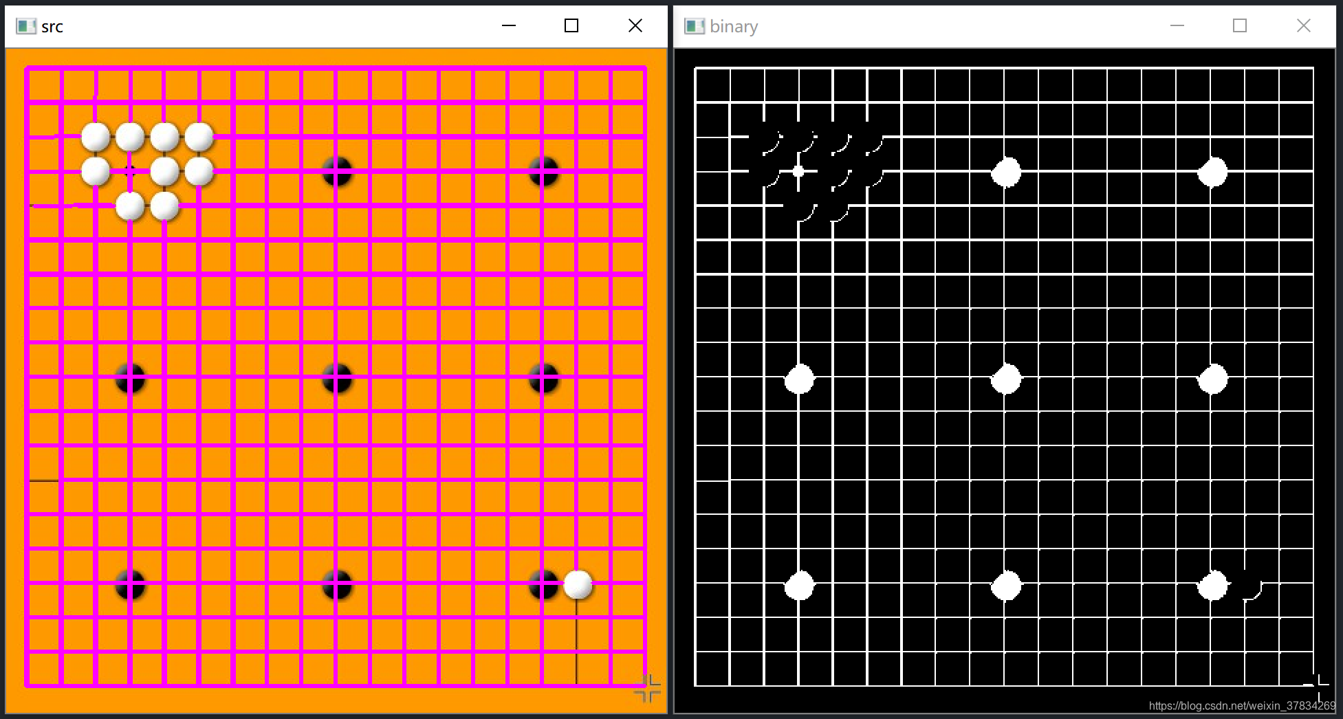
59_查找棋盘上的直线.py

代码

"""
需求：
1. 读取图像，并转化成灰度图
2. 使用 api threshold 将灰度图 二值化
3. 使用 api HoughLinesP 获取 二值图中的 霍夫直线
4. 通过得到的霍夫直线点，在原图同绘制直线
5. 显示图像，等待按键


Each line is represented by a 4-element vector
    .   \f$(x_1, y_1, x_2, y_2)\f$ ,
    where \f$(x_1,y_1)\f$ and \f$(x_2, y_2)\f$ are the ending points of each detected
    .   line segment.
"""

import logging

import cv2 as cv
import numpy as np

logging.basicConfig(level=logging.WARNING)

# 1. 读取图像，并转化成灰度图
filename = r"../img/weiqi.jpg"
src = cv.imread(filename, cv.IMREAD_COLOR)
gray = cv.cvtColor(src, cv.COLOR_BGR2GRAY)

# 2. 使用 api threshold 将灰度图 二值化
_type = cv.THRESH_BINARY_INV
ret_v, binary = cv.threshold(gray, 100, 255, _type)

# 3. 使用 api HoughLinesP 获取 二值图中的 霍夫直线
_rho = 1  # 距离变化的步长  、分辨力
_theta = np.pi / 180  # 弧度变化分辨率
_threshold = 12  # 阈值，一条线段至少要包含10个点
_minLineLength = 25  # 线段以像素为单位的最小长度
_maxLineGap = 3  # 同一方向上两条线段判定为一条线段的最大允许间隔（断裂），超过了设定值，则把两条线段当成一条线段，值越大，允许线段上的断裂越大，越有可能检出潜在的直线段

lines_p = cv.HoughLinesP(binary, rho=_rho, theta=_theta, threshold=_threshold,
                         minLineLength=_minLineLength, maxLineGap=_maxLineGap)
logging.info("lines_p::[{0}]\nshape::{1}".format(lines_p, lines_p.shape))  # shape::(762, 1, 4)

# 4. 通过得到的霍夫直线点，在原图同绘制直线
for line_p in lines_p:
    logging.info(
        "line_p::{0}, line_p.shape{1}".format(line_p, line_p.shape))  # line_p::[[ 96 123  96 123]], line_p.shape(1, 4)
    x1, y1, x2, y2 = line_p[0]
    logging.info("({0}, {1}), ({2}, {3})".format(x1, y1, x2, y2))
    cv.line(src, (x1, y1), (x2, y2), (255, 0, 255), 2)

# 5. 显示图像，等待按键
cv.imshow("src", src)
cv.imshow("binary", binary)

key = cv.waitKey(0)
logging.info("key = [{0}]".format(key))

运行结果
在这里插入图片描述

59_查找棋盘格上的点_滑动条.py

代码

"""
需求：
1. 读取图像，并转化成灰度图
2. 使用 api threshold 将灰度图 二值化
3. 使用 api HoughLinesP 获取 二值图中的 霍夫直线
4. 通过得到的霍夫直线点，在原图同绘制直线
5. 显示图像，等待按键


Each line is represented by a 4-element vector
    .   \f$(x_1, y_1, x_2, y_2)\f$ ,
    where \f$(x_1,y_1)\f$ and \f$(x_2, y_2)\f$ are the ending points of each detected
    .   line segment.
"""

import logging

import cv2 as cv
import numpy as np

logging.basicConfig(level=logging.WARNING)

# 1. 读取图像，并转化成灰度图
filename = r"../img/weiqi.jpg"
src = cv.imread(filename, cv.IMREAD_COLOR)
gray = cv.cvtColor(src, cv.COLOR_BGR2GRAY)

# 2. 使用 api threshold 将灰度图 二值化
_type = cv.THRESH_BINARY_INV
ret_v, binary = cv.threshold(gray, 100, 255, _type)

# 3. 使用 api HoughLinesP 获取 二值图中的 霍夫直线
_rho = 1  # 距离变化的步长  、分辨力
_theta = np.pi / 180  # 弧度变化分辨率
_threshold = 12  # 阈值，一条线段至少要包含10个点
_minLineLength = 25  # 线段以像素为单位的最小长度
_maxLineGap = 3  # 同一方向上两条线段判定为一条线段的最大允许间隔（断裂），超过了设定值，则把两条线段当成一条线段，值越大，允许线段上的断裂越大，越有可能检出潜在的直线段

lines_p = cv.HoughLinesP(binary, rho=_rho, theta=_theta, threshold=_threshold,
                         minLineLength=_minLineLength, maxLineGap=_maxLineGap)
logging.info("lines_p::[{0}]\nshape::{1}".format(lines_p, lines_p.shape))  # shape::(762, 1, 4)

# 4. 通过得到的霍夫直线点，在原图同绘制直线
for line_p in lines_p:
    logging.info(
        "line_p::{0}, line_p.shape{1}".format(line_p, line_p.shape))  # line_p::[[ 96 123  96 123]], line_p.shape(1, 4)
    x1, y1, x2, y2 = line_p[0]
    logging.info("({0}, {1}), ({2}, {3})".format(x1, y1, x2, y2))
    cv.line(src, (x1, y1), (x2, y2), (255, 0, 255), 2)

# 5. 显示图像，等待按键
cv.imshow("src", src)
cv.imshow("binary", binary)

key = cv.waitKey(0)
logging.info("key = [{0}]".format(key))