使用LSTM模型对心跳时间序列数据预测（Python代码，ipynb环境）

所用模块版本：

matplotlib==3.7.1
numpy==1.24.4
pandas==1.5.3
scikit_learn==1.2.2
scipy==1.10.1
seaborn==0.12.2
statsmodels==0.14.0
torch==1.13.1
torch==2.0.1
wfdb==4.1.2

主代码：

import itertools
import pandas as pd
import matplotlib.pyplot as plt
#完整代码：mbd.pub/o/bread/mbd-ZpWUmZ1x


import wfdb
import matplotlib.pyplot as plt

# Specify the path to your downloaded data
path_to_data = 'file_resource/ecg-id-database-1.0.0/Person_03/'

# The record name is the filename without the extension
record_name = 'rec_1'

# Use the 'rdrecord' function to read the ECG data
record = wfdb.rdrecord(f'{path_to_data}/{record_name}')
# Plot the ECG data
plt.figure(figsize=(10, 4))
plt.plot(record.p_signal[:,1])
plt.title('ECG Signal')
plt.xlabel('Time (samples)')
plt.ylabel('Amplitude')
plt.show()
pd.DataFrame(record.p_signal[:,1],columns=["hr"]).to_csv("./P3_rec_1.csv")
hr2 = pd.DataFrame(record.p_signal[:,1],columns=["hr"])[0:10000]
# hr2["index"] = hr2.index


plt.figure(figsize=(10, 4))


from torch import nn
import pandas as pd
import numpy as np
import torch
device = torch.device("cuda" if torch.cuda.is_available() else "cpu")
df = hr2.copy()
df_train = df.loc[:8000].copy()
df_test = df.loc[8000:10000].copy()

target_sensor = "hr"
# features = list(df.columns.difference([target_sensor]))
features = ["hr"]
batch_size =32
forecast_lead = 5
forcast_step = 1
target = f"{target_sensor}_lead{forecast_lead}"

df[target] = df[target_sensor].shift(-forecast_lead)
df = df.iloc[:-forecast_lead]

df_train = df.loc[:8000].copy()
df_test = df.loc[8000-forecast_lead:].copy()

print("Test set fraction:", len(df_train) / len(df_test))

target_mean = df_train[target].mean()
target_stdev = df_train[target].std()
for c in df_train.columns:
    mean = df_train[c].mean()
    stdev = df_train[c].std()

    df_train[c] = (df_train[c] - mean) / stdev
    df_test[c] = (df_test[c] - mean) / stdev
    
    
    
import torch
from torch.utils.data import Dataset

# parse the data into sliding windows
class SequenceDataset(Dataset):
    def __init__(self, dataframe, target, features,sequence_head=10, sequence_length=5):
        self.features = features
        self.target = target
        self.sequence_head = sequence_head
        self.sequence_length = sequence_length
        self.y = torch.tensor(dataframe[target].values).float()
        self.X = torch.tensor(dataframe[features].values).float()

    def __len__(self):
        return self.X.shape[0]-self.sequence_length +1

    def __getitem__(self, i):
        if i >= self.sequence_head - 1:
            i_start = i - self.sequence_head + 1
            x = self.X[i_start:(i + 1), :]

        else:
            padding = self.X[0].repeat(self.sequence_head - i - 1, 1)
            x = self.X[0:(i + 1), :]
            x = torch.cat((padding, x), 0)


        return x.to(device), self.y[i:i+self.sequence_length].to(device)



train_dataset = SequenceDataset(
    df_train,
    target=target,
    features=features,
    sequence_head=forecast_lead,
    sequence_length=forcast_step,

)
    
    
from torch.utils.data import DataLoader
torch.manual_seed(99)

train_loader = DataLoader(train_dataset, batch_size=batch_size, shuffle=False)

for i, (X, y) in enumerate(train_loader):
#     print(X)
    # print(y)
#     print()
    if i >3:break   
    
    from torch.utils.data import DataLoader
torch.manual_seed(99)

    
    
torch.manual_seed(101)

# define the dataset
train_dataset = SequenceDataset(
    df_train,
    target=target,
    features=features,
       sequence_head=forecast_lead,
    sequence_length=forcast_step,
)

test_dataset = SequenceDataset(
    df_test,
    target=target,
    features=["hr"],
    sequence_head=forecast_lead,
    sequence_length=forcast_step,
)

train_loader = DataLoader(train_dataset, batch_size=batch_size, shuffle=True)
test_loader = DataLoader(test_dataset, batch_size=1, shuffle=False)

X, y = next(iter(train_loader))

print("Features shape:", X.shape)
print("Target shape:", y.shape)  
    
    
from torch import nn

# define the model
class ShallowRegressionLSTM(nn.Module):
    def __init__(self, input_size, hidden_size, num_layers, output_size, batch_size):
        super().__init__()
        self.input_size = input_size
        self.hidden_size = hidden_size
        self.num_layers = num_layers
        self.output_size = output_size
        self.num_directions = 1 # 单向LSTM
        self.batch_size = batch_size
        self.lstm = nn.LSTM(self.input_size, self.hidden_size, self.num_layers, batch_first=True)
        self.linear = nn.Linear(self.hidden_size, self.output_size)

    def forward(self, input_seq):
        batch_size, seq_len = input_seq.shape[0], input_seq.shape[1]
        h_0 = torch.randn(self.num_directions * self.num_layers, batch_size, self.hidden_size).to(device)
        c_0 = torch.randn(self.num_directions * self.num_layers, batch_size, self.hidden_size).to(device)
        output, _ = self.lstm(input_seq, (h_0, c_0))
        pred = self.linear(output)
        pred = pred[:, -1, :]
        return pred



class ShallowRegressionRNN(nn.Module):
    def __init__(self, num_sensors, hidden_units):
        super().__init__()
        self.num_sensors = num_sensors  # this is the number of features
        self.hidden_units = hidden_units
        self.num_layers = 1

        self.rnn = nn.RNN(
            input_size=num_sensors,
            hidden_size=hidden_units,
            batch_first=True,
            num_layers=self.num_layers
        )

        self.linear = nn.Linear(in_features=self.hidden_units, out_features=1)

    def forward(self, x):
        batch_size = x.shape[0]
        h0 = torch.zeros(self.num_layers, batch_size, self.hidden_units).requires_grad_().to(device)

        _, hn = self.rnn(x, h0)
        out = self.linear(hn).flatten()

        return out    
    
    
# instantiated the model
num_hidden_units = 512
# loss_function = nn.MSELoss()
model_lstm = ShallowRegressionLSTM(input_size=len(features), hidden_size=num_hidden_units, num_layers=1,output_size=forcast_step,batch_size=batch_size)
class RMSELoss(nn.Module):
    def __init__(self):
        super().__init__()
        self.mse = nn.MSELoss()

    def forward(self,yhat,y):
        return torch.sqrt(self.mse(yhat,y))

loss_function = RMSELoss()
def train_model(data_loader, model, loss_function, optimizer):
    num_batches = len(data_loader)
    total_loss = 0
    model.to(device)
    model.train()

    for X, y in data_loader:
        # print(X.shape)
        output = model(X)
        loss = loss_function(output, y)

        optimizer.zero_grad()
        loss.backward()
        optimizer.step()

        total_loss += loss.item()

    avg_loss = total_loss / num_batches
    print(f"Train loss: {avg_loss}")

def test_model(data_loader, model, loss_function):

    num_batches = len(data_loader)
    total_loss = 0

    model.eval()
    with torch.no_grad():
        for X, y in data_loader:
            output = model(X)
            total_loss += loss_function(output, y).item()

    avg_loss = total_loss / num_batches
    print(f"Test loss: {avg_loss}")
    return avg_loss


print("Untrained test\n--------")
# test_model(test_loader, model, loss_function)

avg_loss = 1
model_lstm.to(device)    
    
    
learning_rate = 5e-4
# train the model
optimizer = torch.optim.Adam(model_lstm.parameters(), lr=learning_rate)
for ix_epoch in range(150):
    print(f"Epoch {ix_epoch}\n---------")
    train_model(train_loader, model_lstm, loss_function, optimizer=optimizer)
    temp = test_model(test_loader, model_lstm, loss_function)
    if temp < avg_loss:
        avg_loss = temp
        torch.save(model_lstm.state_dict(), "model_lstm_%s_%s.pt"% (forecast_lead,forcast_step))
    # if ix_epoch % 20 == 0:
    #     learning_rate = learning_rate * 0.6
    #     optimizer = torch.optim.Adam(model_lstm.parameters(), lr=learning_rate)
    #     print(learning_rate)
    print()    
    
    
    
# save the model
# torch.save(model_lstm.state_dict(), "model_lstm.pt")

model_lstm.load_state_dict(torch.load("model_lstm_%s_%s.pt"% (forecast_lead,forcast_step)))    
    
# predict the model
def predict(data_loader, model):

    output = torch.tensor([]).to(device)
    model.eval()
    with torch.no_grad():
        for X, _ in data_loader:
            y_star = model(X)
            output = torch.cat((output, y_star), 0)

    return output


train_eval_loader = DataLoader(train_dataset, batch_size=batch_size, shuffle=False)

ystar_col = "Model forecast"
pre = predict(train_eval_loader, model_lstm).cpu().numpy()
print(pre.shape)
df_train[ystar_col] = predict(train_eval_loader, model_lstm).cpu().numpy()
df_test[ystar_col] = predict(test_loader, model_lstm).cpu().numpy()

df_out = pd.concat((df_train, df_test))[[target, ystar_col]]



for c in df_out.columns:
    df_out[c] = df_out[c] * target_stdev + target_mean

print(df_out)
    
    
# use last predict data to be the next input
def predict_window(data_loader, model, forecast_step=2000):
    output = torch.tensor([]).to(device)
    model.eval()
    count = 0
    with torch.no_grad():
        for X, _ in data_loader:
            y_star = model(X)
            output = torch.cat((output, y_star), 0)
            count +=1
            # print(X)
            if count > forecast_lead:
                break
        for i in range(forecast_step-1):
            y_star = model(output[output.shape[0]-forecast_lead:].reshape(1,forecast_lead,1))
            print(output)
            print(output[output.shape[0]-forecast_lead:])
            # y_star = model(output.reshape(1,forecast_lead,1))
            output = torch.cat((output, y_star), 0)
            if i > 10:
                break

    return output
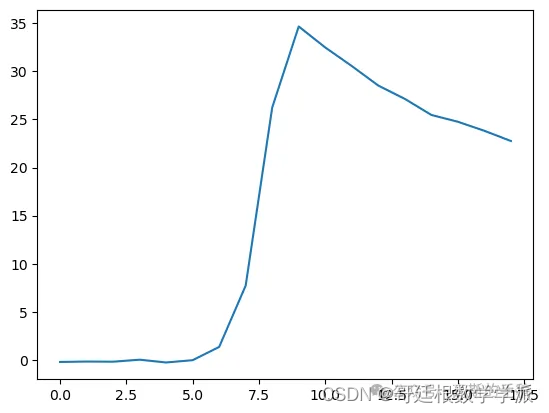
res = predict_window(test_loader, model_lstm).cpu().numpy()
print(res)
plt.plot(res)



import matplotlib.pyplot as plt
from sklearn.metrics import mean_absolute_error, mean_squared_error, r2_score,mean_absolute_percentage_error
fig, ax = plt.subplots(figsize=(12, 6))
df_out[8000:].plot(ax=ax)
ax.set_title("LSTM model forecast")
ax.set_ylabel("ECG")
ax.set_xlabel("Time")
plt.show()

# calculate the  error
# calculate the  AIC
from sklearn.metrics import mean_absolute_error, mean_squared_error, r2_score,mean_absolute_percentage_error

def calculate_aic(y_true, y_pred, num_params):
    mse = mean_squared_error(y_true, y_pred)
    aic = len(y_true) * np.log(mse) + 2 * num_params
    return aic

mse = mean_squared_error(df_out[target], df_out[ystar_col])
mae = mean_absolute_error(df_out[target], df_out[ystar_col])
r2 = r2_score(df_out[target], df_out[ystar_col])
mape = mean_absolute_percentage_error(df_out[target], df_out[ystar_col])
print(f"R2: {r2:.6f}")
print(f"MAPE: {mape:.6f}")
print(f"MAE: {mae:.6f} ")
print(f"RMSE: {np.sqrt(mse):.6f}")
print(f"mse: {mse:.6f}")
print(f"AIC: {calculate_aic(df_out[target], df_out[ystar_col], 1):.6f}")


num_hidden_units = 128
# use sdg loss
loss_function = nn.MSELoss()
model = ShallowRegressionRNN(num_sensors=len(features), hidden_units=num_hidden_units)
model.to(device)
avg_loss = 1
# loss_function = RMSELoss()

learning_rate = 1e-4

optimizer = torch.optim.Adam(model.parameters(), lr=learning_rate)
for ix_epoch in range(500):
    print(f"Epoch {ix_epoch}\n---------")
    train_model(train_loader, model, loss_function, optimizer=optimizer)
    temp = test_model(test_loader, model, loss_function)
    if temp < avg_loss:
        avg_loss = temp
        torch.save(model.state_dict(), "model_RNN.pt")
    print()

# save the model
# torch.save(model.state_dict(), "model_RNN.pt")

# load the model
model.load_state_dict(torch.load("model_RNN.pt"))
print(avg_loss)


res = predict_window(test_loader, model).cpu().numpy()
print(len(res))
plt.plot(res)

def predict(data_loader, model):

    output = torch.tensor([]).to(device)
    model.eval()
    with torch.no_grad():
        for X, _ in data_loader:
            y_star = model(X)
            output = torch.cat((output, y_star), 0)

    return output


train_eval_loader = DataLoader(train_dataset, batch_size=batch_size, shuffle=False)

ystar_col = "Model forecast"
df_train[ystar_col] = predict(train_eval_loader, model).cpu().numpy()
df_test[ystar_col] = predict(test_loader, model).cpu().numpy()

df_out = pd.concat((df_train, df_test))[[target, ystar_col]]

# for c in df_out.columns:
#     df_out[c] = df_out[c] * target_stdev + target_mean

print(df_out)

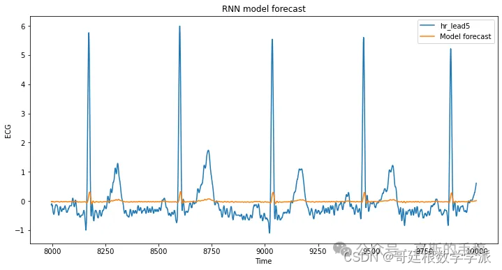
import matplotlib.pyplot as plt

fig, ax = plt.subplots(figsize=(12, 6))
df_out[8000:].plot(ax=ax)
ax.set_title("RNN model forecast")
ax.set_ylabel("ECG")
ax.set_xlabel("Time")
plt.show()


from sklearn.metrics import mean_absolute_error, mean_squared_error, r2_score,mean_absolute_percentage_error
mse = mean_squared_error(df_out[target], df_out[ystar_col])
mae = mean_absolute_error(df_out[target], df_out[ystar_col])
r2 = r2_score(df_out[target], df_out[ystar_col])
mape = mean_absolute_percentage_error(df_out[target], df_out[ystar_col])
print(f"R2: {r2:.6f}")
print(f"MAPE: {mape:.6f}")
print(f"MAE: {mae:.6f} ")
print(f"RMSE: {np.sqrt(mse):.6f}")
print(f"mse: {mse:.6f}")
print(f"AIC: {calculate_aic(df_out[target], df_out[ystar_col], 1):.6f}")
# aic_res = calaic(df_out[target], df_out[ystar_col], df_out.shape[1])
# print(f"AIC: {aic_res:.6f}")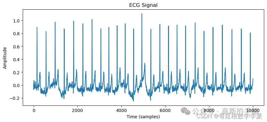

工学博士，担任《Mechanical System and Signal Processing》等期刊审稿专家，擅长领域：现代信号处理，机器学习，深度学习，数字孪生，时间序列分析，设备缺陷检测、设备异常检测、设备智能故障诊断与健康管理PHM等。