人工神经网络_制作属于自己的人工神经网络

最新推荐文章于 2024-04-24 18:02:35 发布

weixin_39667626

最新推荐文章于 2024-04-24 18:02:35 发布

阅读量323

点赞数

文章标签：人工神经网络

本文链接：https://blog.csdn.net/weixin_39667626/article/details/111376361

版权

在本文中，我已经实现了具有Dropout和L2正则化的人工神经网络的完全向量化代码。

在本文中，我实现了一个在多个数据集上测试的人工神经网络的完全向量化python代码。此外，并对Dropout和L2正则化技术进行了实现和详细说明。

强烈建议通过人工神经网络的基本工作，正向传播和反向传播。

本文分为10个部分：

介绍
先决条件
导入我们的库
激活函数及求导
神经网络类
初始化权重和偏差
正向传播
成本函数
反向传播
预测新数据集的标签

1.简介

人工神经网络是监督深度学习中最简单和最基本的概念之一。它可用于执行多个任务，如二进制或分类。它看起来很容易理解和实现。在编写这样一个网络的过程中，会出现一些小问题，这些问题会导致很大的错误，并帮助您理解以前忽略的概念。因此，在本文中，我尝试实现一个人工神经网络，它可能会帮助您节省正确编码和理解主题的每个概念所需的工作时间。

2.先决条件

我假设你知道神经网络是什么以及它们是如何学习的。如果你对Python和像numpy这样的库很熟悉的话，这将很容易理解。另外，还需要对线性代数和微积分知识有很好的了解，以便于轻松地理解正向和反向传播部分。此外，我强烈建议您阅读Andrew Ng在Coursera上的课程视频(https://www.coursera.org/ ； https://www.deeplearning.ai/ )。

3.导入我们的库

现在，我们可以开始对神经网络进行编码了。第一件事是需要导入我们实现网络所需的所有库。

# Importing the librariesimport numpy as npimport matplotlib.pyplot as pltimport pandas as pdimport warningsimport timewarnings.filterwarnings('ignore');import osimport sys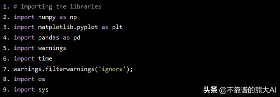

我们将使用pandas导入和清理我们的数据集。Numpy 是执行矩阵代数和复杂计算的最重要的库。

4.激活函数及求导

在本文后面的部分中，我们将需要激活函数来执行正向传播。另外，我们还需要在反向传播过程中对激活函数求导。

所以，让我们编写一些激活函数。

def sigmoid(z) : """ Reutrns the element wise sigmoid function. """ return 1./(1 + np.exp(-z))def sigmoid_prime(z) : """ Returns the derivative of the sigmoid function. """ return sigmoid(z)*(1-sigmoid(z))def ReLU(z) :  """ Reutrns the element wise ReLU function. """ return (z*(z > 0))def ReLU_prime(z) : """ Returns the derivative of the ReLU function. """ return 1*(z>=0)def lReLU(z) :  """ Reutrns the element wise leaky ReLU function. """ return np.maximum(z/100,z)def lReLU_prime(z) : """ Returns the derivative of the leaky ReLU function. """ z = 1*(z>=0) z[z==0] = 1/100 return zdef tanh(z) : """ Reutrns the element wise hyperbolic tangent function. """ return np.tanh(z)def tanh_prime(z) :  """ Returns the derivative of the tanh function. """ return (1-tanh(z)**2)# A dictionary of our activation functionsPHI = {'sigmoid':sigmoid, 'relu':ReLU, 'lrelu':lReLU, 'tanh':tanh}# A dictionary containing the derivatives of our activation functionsPHI_PRIME = {'sigmoid':sigmoid_prime, 'relu':ReLU_prime, 'lrelu':lReLU_prime, 'tanh':tanh_prime}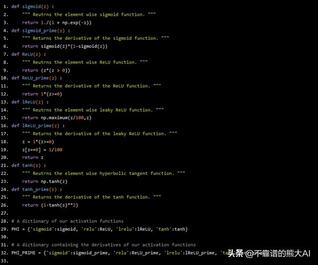

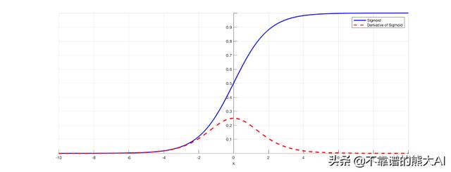
我们有四种最流行的激活函数。首先是常规的sigmoid激活函数。

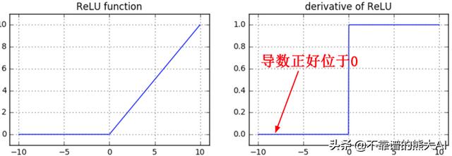
我们有ReLU或“ 线性整流函数 ”。我们将主要使用这个激活函数。注意，我们将保持ReLU 0的导数在点0处。

我们还有一个ReLU的扩展版本叫做Leaky ReLU。它的工作原理与ReLU类似，可以在某些数据集上提供更好的结果(不一定是全部)。

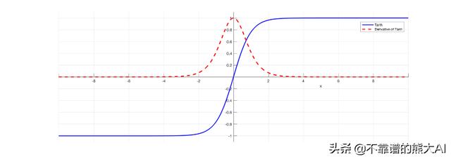
我们还有tanh(双曲正切)激活函数。它也被广泛使用，并且几乎总是优于sigmoid。

另外，PHI和PHI_PRIME是分别包含激活函数及其导数的python字典。

5.我们的神经网络类

在本节中，我们将创建并初始化我们的神经网络类。首先，我们将决定在初始化期间使用哪些参数。我们需要：

每层神经元的数量
我们想在每一层中使用激活函数
我们的特征矩阵(X包含行特征和列特征)。
特征矩阵对应的标签(y是行向量)
初始化权重和偏差的方法
使用损失函数

记住这一点，让我们开始编写神经网络的类：

class NeuralNet :  """ This is a class for making Artificial Neural Networks. L2 and Droupout are the  default regularization methods implemented in this class. It takes the following parameters:  1. layers : A python list containing the different number of neurons in each layer. (containing the output layer) Eg - [64,32,16,16,1]  2. X : Matrix of features with rows as features and columns as different examples.  3. y : Numpy array containing the ouputs of coresponding examples.  4. ac_funcs : A python list containing activation function of each layer. Eg - ['relu','relu','lrelu','tanh','sigmoid']  5. init_method : Meathod to initialize weights of the network. Can be 'gaussian','random','zeros'.  6. loss_func : Currently not implemented  7. W : Weights of a pretrained neural network with same architecture.  8. W : Biases of a pretrained neural network with same architecture. """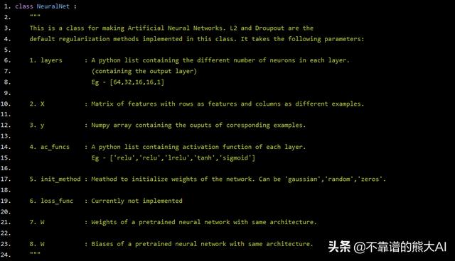

现在我们有了一个正确记录的神经网络类，我们可以继续初始化网络的其他变量。

 def __init__(self, layers, X, y, ac_funcs, init_method='gaussian', loss_func='b_ce', W=np.array([]), B=np.array([])) : """ Initialize the network. """ # Store the layers of the network self.layers = layers # ---- self.W = None self.B = None # Store the number of examples in the dataset as m self.m = X.shape[1] # Store the full layer list as n self.n = [X.shape[0], *layers] # Save the dataset self.X = X # Save coresponding output self.y = y # List to store the cost of the model calculated during training self.cost = [] # Stores the accuracy obtained on the test set. self.acc = 0 # Activation function of each layer self.ac_funcs = ac_funcs self.loss = loss_func # Inittialize the weights by provided methods if not provided.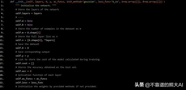

我们将使用' self.m'来存储数据集中示例的数量。' self.n '将存储每层中神经元数量的信息。' self.ac_funcs '是每层的激活函数的python列表。' self.cost '将在我们训练网络时存储成本函数的记录值。' self.acc '将在训练后的数据集上存储记录的精度。在初始化网络的所有变量之后，让我们进一步初始化网络的权重和偏差。

6.初始化权重和偏差

我们知道权重不能初始化为零，因为每个神经元的假设变得相同而网络永远不会学习。因此，我们必须有一些方法来使我们的神经网络学习。我们可以使用高斯正态分布来获得随机值。由于这些分布的均值为零，因此权重集中在零并且非常小。因此，网络开始非常快速有效地学习。我们可以使用np.random.randn()函数从正态分布中生成随机值。

 # Inittialize the weights by provided methods if not provided. if len(W) and len(B) : self.W = W self.B = B else :  if init_method=='gaussian':  self.W = [np.random.randn(self.n[nl], self.n[nl-1]) for nl in range(1,len(self.n))] self.B = [np.zeros((nl,1), 'float32') for nl in self.layers] elif init_method == 'random': self.W = [np.random.rand(self.n[nl], self.n[nl-1]) for nl in range(1,len(self.n))] self.B = [np.random.rand(nl,1) for nl in self.layers] elif init_method == 'zeros': self.W = [np.zeros((self.n[nl], self.n[nl-1]), 'float32') for nl in range(1,len(self.n))] self.B = [np.zeros((nl,1), 'float32') for nl in self.layers]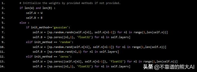

我们已将权重初始化为正态分布中的随机值。偏差已初始化为零。

7.正向传播

首先，让我们理解没有正则化的正向传播。

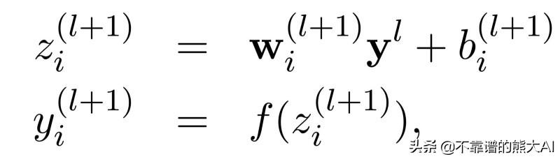
我们用Z表示每个神经元从一层到另一层的连接。一旦我们计算了Z，我们将激活函数f应用于Z值以获得每层中每个神经元的激活y。这是简单的正向传播。Dropout是一种提高神经网络泛化能力和鲁棒性的神奇技术。所以，让我们首先了解一下Dropout正则化。

Dropout正则化的本质

Dropout，顾名思义，是指神经网络中的一些神经元“失活”，并对其余的神经元进行训练。

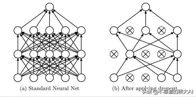
为了提高性能，我们可以训练几十个和几百个具有不同超参数值的神经网络，获得所有网络的输出并取其平均值来获得最终结果。这个过程在计算上非常昂贵并且实际上不能实现。因此，我们需要一种以更优化和计算成本更低的方式执行类似操作的方法。Dropout正则化以非常便宜和简单的方式完成相似的事情。事实上，Dropout是优化性能的简单方法，近年来受到了广泛的关注，并且几乎在许多其他深度学习模型中无处不在。

要实现Dropout，我们将使用以下方法：

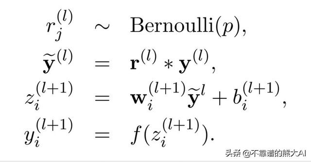
我们将首先从伯努利分布中提取随机值，如果概率高于某个阈值则保持神经元不变，然后执行常规正向传播。注意，我们不会在预测新数据集上的值或测试时间期间应用dropout。

实现Dropout的代码

我们使用keep_prob作为每层神经元存活的概率。我们只保留概率高于存活概率或keep_prob的神经元。假设，它的值是0.8。这意味着我们将使每一层中20%的神经元失活，并训练其余80%的神经元。注意，我们在每次迭代后停用随机选择的神经元。这有助于神经元学习在更大的数据集上泛化的特征。

 def _feedForward(self, keep_prob): """ Forward pass """ z = [];a = [] z.append(np.dot(self.W[0], self.X) + self.B[0]) a.append(PHI[self.ac_funcs[0]](z[-1])) for l in range(1,len(self.layers)): z.append(np.dot(self.W[l], a[-1]) + self.B[l]) # a.append(PHI[self.ac_funcs[l]](z[l])) _a = PHI[self.ac_funcs[l]](z[l]) a.append( ((np.random.rand(_a.shape[0],1) < keep_prob)*_a)/keep_prob ) return z,a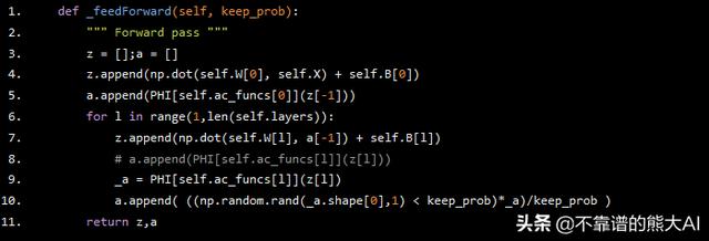

我们首先初始化将存储Z和A值的列表。我们首先在Z中附加第一层的线性值，然后在A中附加第一层神经元的激活。PHI是一个python字典，包含我们之前编写的激活函数。类似地使用for循环计算所有其他层的Z和A的值。注意，我们没有在输入层应用dropout。我们最终返回Z和A的计算值。

8.成本函数

我们将使用标准二进制/分类交叉熵成本函数。

 def _cost_func(self, a, _lambda): """ Binary Cross Entropy Cost Function """ return ( (-1/self.m)*np.sum(np.nan_to_num(self.y*np.log(a) + (1-self.y)*np.log(1-a))) + (_lambda/(2*self.m))*np.sum([np.sum(i**2) for i in self.W]) ) def _cost_derivative(self, a) :  """ The derivative of cost w.r.t z """ return (a-self.y)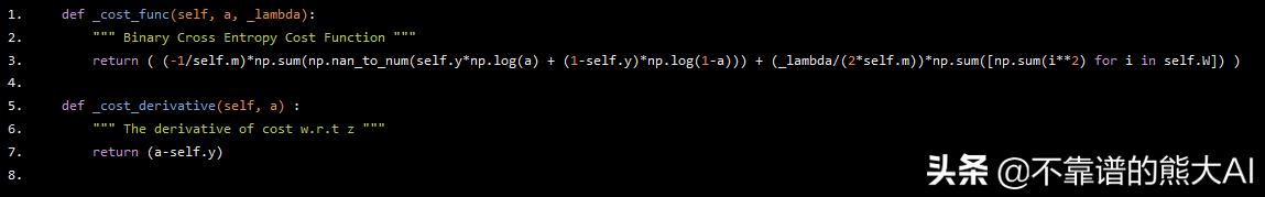

我们用L2正则化对我们的成本函数进行了编译。lambda参数称为“ 惩罚参数 ”。它有助于使权重值不会迅速增加，从而更好地形成。这里，' a'包含输出层的激活值。我们还有函数_cost_derivative来计算成本函数对输出层激活的导数。我们稍后会在反向传播期间使用它。

9.反向传播

以下是我们需要执行反向传播的一些公式。

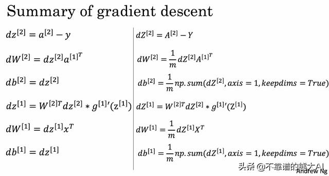
我们将在深度神经网络上实现这一点。右边的公式是完全向量化的。一旦理解了这些公式，我们就可以继续对它们进行编译。

 def startTraining(self, epochs, alpha, _lambda, keep_prob=0.5, interval=100): """ Start training the neural network. It takes the followng parameters :   1. epochs : Number of epochs for which you want to train the network.  2. alpha : The learning rate of your network.  3. _lambda : L2 regularization parameter or the penalization parameter.  4. keep_prob : Dropout regularization parameter. The probability of neurons to deactivate. Eg - 0.8 means 20% of the neurons have been deactivated.  5. interval : The interval between updates of cost and accuracy. """ start = time.time() for i in range(epochs+1) :  z,a = self._feedForward(keep_prob) delta = self._cost_derivative(a[-1]) for l in range(1,len(z)) :  delta_w = np.dot(delta, a[-l-1].T) + (_lambda)*self.W[-l] delta_b = np.sum(delta, axis=1, keepdims=True) delta = np.dot(self.W[-l].T, delta)*PHI_PRIME[self.ac_funcs[-l-1]](z[-l-1]) self.W[-l] = self.W[-l] - (alpha/self.m)*delta_w self.B[-l] = self.B[-l] - (alpha/self.m)*delta_b delta_w = np.dot(delta, self.X.T ) + (_lambda)*self.W[0] delta_b = np.sum(delta, axis=1, keepdims=True) self.W[0] = self.W[0] - (alpha/self.m)*delta_w self.B[0] = self.B[0] - (alpha/self.m)*delta_b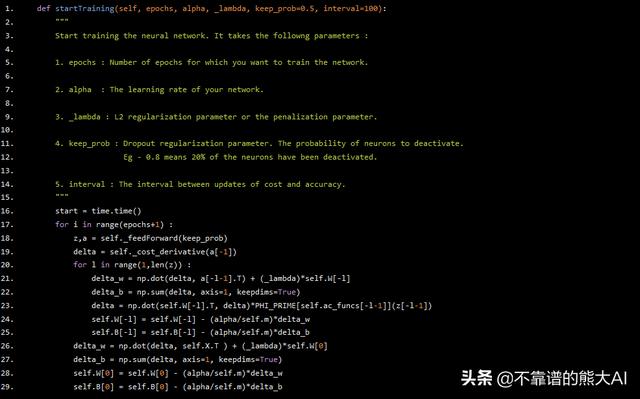

我们将epochs、alpha(学习率)、_lambda、keep_prob和interval作为函数的参数来实现反向传播。

我们从正向传播开始。然后我们将成本函数的导数计算为delta。现在，对于每一层，我们计算delta_w和delta_b，其中包含成本函数对网络的权重和偏差的导数。然后我们根据各自的公式更新delta，权重和偏差。在将最后一层的权重和偏差更新到第二层之后，我们更新第一层的权重和偏差。我们这样做了几次迭代，直到权重和偏差的值收敛。

重要提示：此处可能出现的一个重大错误是在更新权重和偏差后更新delta 。这样做可能会导致非常糟糕的梯度渐变消失/爆炸问题。

我们的大部分工作都在这里完成，但是我们仍然需要编译可以预测新数据集结果的函数。因此，作为我们的最后一步，我们将编写一个函数来预测新数据集的标签。

10.预测新数据集的标签

这一步非常简单。我们只需要执行正向传播但不需要Dropout正则化。我们不需要在测试时应用Dropout正则化，因为我们需要所有层的所有神经元来为我们提供适当的结果，而不仅仅是一些随机值。

 def predict(self, X_test) : """ Predict the labels for a new dataset. Returns probability. """ a = PHI[self.ac_funcs[0]](np.dot(self.W[0], X_test) + self.B[0]) for l in range(1,len(self.layers)): a = PHI[self.ac_funcs[l]](np.dot(self.W[l], a) + self.B[l]) return a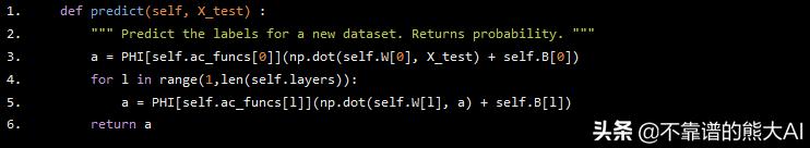

我们将返回输出层的激活作为结果。

整个代码

以下是您自己实现人工神经网络的完整代码。我在培训时添加了一些代码来打印网络的成本和准确性。除此之外，一切都是一样的。

# Importing the librariesimport numpy as npimport matplotlib.pyplot as pltimport pandas as pdimport warningsimport timewarnings.filterwarnings('ignore');import osimport sys# Importing our datasetos.chdir("C:/Users/Hilak/Desktop/INTERESTS/Machine Learning A-Z Template Folder/Part 3 - Classification/Section 14 - Logistic Regression");training_set = pd.read_csv("Social_Network_Ads.csv");# Splitting our dataset into matrix of features and output values.X = training_set.iloc[:, 1:4].valuesy = training_set.iloc[:, 4].values# Encoding our object features.from sklearn.preprocessing import LabelEncoder, OneHotEncoderle_x = LabelEncoder()X[:,0] = le_x.fit_transform(X[:,0])ohe = OneHotEncoder(categorical_features = [0])X = ohe.fit_transform(X).toarray()# Performing Feature scalingfrom sklearn.preprocessing import StandardScalerss = StandardScaler()X[:,2:4] = ss.fit_transform(X[:, 2:4])# Splitting the dataset into train and test set.from sklearn.model_selection import train_test_splitX_train, X_test, y_train, y_test = train_test_split(X,y,test_size=0.3)X_train = X_train.TX_test = X_test.T# # Alternate Dataset for test purposes. Not used in the example shown# os.chdir("C:甥敳獲HilakDesktopINTERESTSMachine Learning A-Z Template FolderPart 8 - Deep LearningSection 39 - Artificial Neural Networks (ANN)");# dataset = pd.read_csv('Churn_Modelling.csv')# X = dataset.iloc[:, 3:13].values# y = dataset.iloc[:, 13].values# # Encoding categorical data# from sklearn.preprocessing import LabelEncoder, OneHotEncoder# labelencoder_X_1 = LabelEncoder()# X[:, 1] = labelencoder_X_1.fit_transform(X[:, 1])# labelencoder_X_2 = LabelEncoder()# X[:, 2] = labelencoder_X_2.fit_transform(X[:, 2])# onehotencoder = OneHotEncoder(categorical_features = [1])# X = onehotencoder.fit_transform(X).toarray()# X = X[:, 1:]# # Splitting the dataset into the Training set and Test set# from sklearn.model_selection import train_test_split# X_train, X_test, y_train, y_test = train_test_split(X, y, test_size = 0.2)# X_test, X_CV, y_test, y_CV = train_test_split(X, y, test_size = 0.5)# # Feature Scaling# from sklearn.preprocessing import StandardScaler# sc = StandardScaler()# X_train = sc.fit_transform(X_train)# X_test = sc.transform(X_test)# X_train = X_train.T# X_test = X_test.T# X_CV = X_CV.Tdef sigmoid(z) : """ Reutrns the element wise sigmoid function. """ return 1./(1 + np.exp(-z))def sigmoid_prime(z) : """ Returns the derivative of the sigmoid function. """ return sigmoid(z)*(1-sigmoid(z))def ReLU(z) :  """ Reutrns the element wise ReLU function. """ return (z*(z > 0))def ReLU_prime(z) : """ Returns the derivative of the ReLU function. """ return 1*(z>=0)def lReLU(z) :  """ Reutrns the element wise leaky ReLU function. """ return np.maximum(z/100,z)def lReLU_prime(z) : """ Returns the derivative of the leaky ReLU function. """ z = 1*(z>=0) z[z==0] = 1/100 return zdef tanh(z) : """ Reutrns the element wise hyperbolic tangent function. """ return np.tanh(z)def tanh_prime(z) :  """ Returns the derivative of the tanh function. """ return (1-tanh(z)**2)# A dictionary of our activation functionsPHI = {'sigmoid':sigmoid, 'relu':ReLU, 'lrelu':lReLU, 'tanh':tanh}# A dictionary containing the derivatives of our activation functionsPHI_PRIME = {'sigmoid':sigmoid_prime, 'relu':ReLU_prime, 'lrelu':lReLU_prime, 'tanh':tanh_prime}class NeuralNet :  """ This is a class for making Artificial Neural Networks. L2 and Droupout are the  default regularization methods implemented in this class. It takes the following parameters:  1. layers : A python list containing the different number of neurons in each layer. (containing the output layer) Eg - [64,32,16,16,1]  2. X : Matrix of features with rows as features and columns as different examples.  3. y : Numpy array containing the ouputs of coresponding examples.  4. ac_funcs : A python list containing activation function of each layer. Eg - ['relu','relu','lrelu','tanh','sigmoid']  5. init_method : Meathod to initialize weights of the network. Can be 'gaussian','random','zeros'.  6. loss_func : Currently not implemented  7. W : Weights of a pretrained neural network with same architecture.  8. W : Biases of a pretrained neural network with same architecture. """ def __init__(self, layers, X, y, ac_funcs, init_method='gaussian', loss_func='b_ce', W=np.array([]), B=np.array([])) : """ Initialize the network. """ # Store the layers of the network self.layers = layers # ---- self.W = None self.B = None # Store the number of examples in the dataset as m self.m = X.shape[1] # Store the full layer list as n self.n = [X.shape[0], *layers] # Save the dataset self.X = X # Save coresponding output self.y = y # List to store the cost of the model calculated during training self.cost = [] # Stores the accuracy obtained on the test set. self.acc = 0 # Activation function of each layer self.ac_funcs = ac_funcs self.loss = loss_func # Inittialize the weights by provided methods if not provided. if len(W) and len(B) : self.W = W self.B = B else :  if init_method=='gaussian':  self.W = [np.random.randn(self.n[nl], self.n[nl-1]) for nl in range(1,len(self.n))] self.B = [np.zeros((nl,1), 'float32') for nl in self.layers] elif init_method == 'random': self.W = [np.random.rand(self.n[nl], self.n[nl-1]) for nl in range(1,len(self.n))] self.B = [np.random.rand(nl,1) for nl in self.layers] elif init_method == 'zeros': self.W = [np.zeros((self.n[nl], self.n[nl-1]), 'float32') for nl in range(1,len(self.n))] self.B = [np.zeros((nl,1), 'float32') for nl in self.layers]  def startTraining(self, epochs, alpha, _lambda, keep_prob=0.5, interval=100): """ Start training the neural network. It takes the followng parameters :   1. epochs : Number of epochs for which you want to train the network.  2. alpha : The learning rate of your network.  3. _lambda : L2 regularization parameter or the penalization parameter.  4. keep_prob : Dropout regularization parameter. The probability of neurons to deactivate. Eg - 0.8 means 20% of the neurons have been deactivated.  5. interval : The interval between updates of cost and accuracy. """ start = time.time() for i in range(epochs+1) :  z,a = self._feedForward(keep_prob) delta = self._cost_derivative(a[-1]) for l in range(1,len(z)) :  delta_w = np.dot(delta, a[-l-1].T) + (_lambda)*self.W[-l] delta_b = np.sum(delta, axis=1, keepdims=True) delta = np.dot(self.W[-l].T, delta)*PHI_PRIME[self.ac_funcs[-l-1]](z[-l-1]) self.W[-l] = self.W[-l] - (alpha/self.m)*delta_w self.B[-l] = self.B[-l] - (alpha/self.m)*delta_b delta_w = np.dot(delta, self.X.T ) + (_lambda)*self.W[0] delta_b = np.sum(delta, axis=1, keepdims=True) self.W[0] = self.W[0] - (alpha/self.m)*delta_w self.B[0] = self.B[0] - (alpha/self.m)*delta_b if not i%interval : aa = self.predict(self.X) if self.loss == 'b_ce': aa = aa > 0.5 self.acc = sum(sum(aa == self.y)) / self.m cost_val = self._cost_func(a[-1], _lambda) self.cost.append(cost_val) elif self.loss == 'c_ce': aa = np.argmax(aa, axis = 0) yy = np.argmax(self.y, axis = 0) self.acc = np.sum(aa==yy)/(self.m) cost_val = self._cost_func(a[-1], _lambda) self.cost.append(cost_val) sys.stdout.write(f'Epoch[{i}] : Cost = {cost_val:.2f} ; Acc = {(self.acc*100):.2f}% ; Time Taken = {(time.time()-start):.2f}s') print('') return None  def predict(self, X_test) : """ Predict the labels for a new dataset. Returns probability. """ a = PHI[self.ac_funcs[0]](np.dot(self.W[0], X_test) + self.B[0]) for l in range(1,len(self.layers)): a = PHI[self.ac_funcs[l]](np.dot(self.W[l], a) + self.B[l]) return a   def _feedForward(self, keep_prob): """ Forward pass """ z = [];a = [] z.append(np.dot(self.W[0], self.X) + self.B[0]) a.append(PHI[self.ac_funcs[0]](z[-1])) for l in range(1,len(self.layers)): z.append(np.dot(self.W[l], a[-1]) + self.B[l]) # a.append(PHI[self.ac_funcs[l]](z[l])) _a = PHI[self.ac_funcs[l]](z[l]) a.append( ((np.random.rand(_a.shape[0],1) < keep_prob)*_a)/keep_prob ) return z,a  def _cost_func(self, a, _lambda): """ Binary Cross Entropy Cost Function """ return ( (-1/self.m)*np.sum(np.nan_to_num(self.y*np.log(a) + (1-self.y)*np.log(1-a))) + (_lambda/(2*self.m))*np.sum([np.sum(i**2) for i in self.W]) ) def _cost_derivative(self, a) :  """ The derivative of cost w.r.t z """ return (a-self.y)  @property def summary(self) : return self.cost, self.acc, self.W,self.B def __repr__(self) :  return f''# Initializing our neural networkneural_net_sigmoid = NeuralNet([32,16,1], X_train, y_train, ac_funcs = ['relu','relu','sigmoid'])# Staring the training of our network.neural_net_sigmoid.startTraining(5000, 0.01, 0.2, 0.5, 100)# Predicting on new dataset using our trained network.preds = neural_net_sigmoid.predict(X_test)preds = preds > 0.5acc = (sum(sum(preds == y_test)) / y_test.size)*100# Accuracy (metric of evaluation) obtained by the network.print(f'Test set Accuracy ( r-t-s ) : {acc}%')# Plotting our cost vs epochs relationshipsigmoid_summary = neural_net_sigmoid.summaryplt.plot(range(len(sigmoid_summary[0])), sigmoid_summary[0], label='Sigmoid Cost')plt.title('Cost')plt.show()# Comparing our results with the library keras.from keras.models import Sequentialfrom keras.layers import DenseX_train, X_test = X_train.T, X_test.Tclassifier = Sequential()classifier.add(Dense(input_dim=4, units = 32, kernel_initializer="uniform