mae python实现_Python机器学习（十）经典算法大全

1.KNN 分类算法

由于knn算法涉及到距离的概念，KNN 算法需要先进行归一化处理

1.1 归一化处理 scaler

from sklearn.preprocessing importStandardScaler

standardScaler=StandardScaler()

standardScaler.fit(X_train)

X_train_standard=standardScaler.transform(X_train)

X_test_standard= standardScaler.transform(X_test)

归一化之后送入模型进行训练

from sklearn.neighbors importKNeighborsClassifier

knn_clf= KNeighborsClassifier(n_neighbors=8)

knn_classifier.fit(X_train_standard, y_train)

y_predict=knn_clf.predict(X_test_standard)#默认的预测指标为分类准确度

knn_clf.score(X_test, y_test)

1.2 网格搜索 GridSearchCV

使用网格搜索来确定KNN算法合适的超参数

from sklearn.model_selection importGridSearchCV

param_grid=[

{

‘weights‘:[‘uniform‘],

‘n_neighbors‘:[ ifor i in range(1, 11)]

},

{

‘weights‘:[‘distance‘],

‘n_neighbors‘:[ifor i in range(1, 11)],

‘p‘:[pfor p in range(1, 6)]

}

]

grid_search= GridSearchCV(knn_clf, param_grid, n_jobs=-1, verbose=2)

grid_search.fit(X_train_standard, y_train)

knn_clf=grid_search.best_estimator_

knn_clf.score(X_test_standard, y_test)

1.3 交叉验证

GridSearchCV 本身就包括了交叉验证，也可自己指定参数cv

默认GridSearchCV的KFold平分为3份

自己指定交叉验证，查看交叉验证成绩

from sklearn.model_selection importcross_val_score#默认为分成3份

cross_val_score(knn_clf, X_train, y_train, cv=5)

这里默认的scoring标准为 accuracy

有许多可选的参数，具体查看官方文档

封装成函数，在fit完模型之后，一次性查看多个评价指标的成绩

这里选的只是针对分类算法的指标，也可以是针对回归，聚类算法的评价指标

defcv_score_train_test(model):

num_cv= 5score_list= ["accuracy","f1", "neg_log_loss", "roc_auc"]for score inscore_list:print(score,"\t train:",cross_val_score(model, X_train, y_train, cv=num_cv, scoring=score).mean())print(score,"\t test:",cross_val_score(model, X_test, y_test, cv=num_cv, scoring=score).mean())

2. 线性回归

2.1 简单线性回归

from sklearn.linear_model importLinearRegression

linreg=LinearRegression()

linreg.fit(X_train, y_train)

#查看截距和系数printlinreg.intercept_printlinreg.coef_

lin_reg.score(X_test, y_test)

y_predict= linreg.predict(X_test)

2.2 多元线性回归

在更高维度的空间中的“直线”，即数据不只有一个维度，而具有多个维度

代码和上面的简单线性回归相同

3. 梯度下降法

使用梯度下降法之前，需要对数据进行归一化处理

3.1 随机梯度下降线性回归

SGD_reg

from sklearn.linear_model importSGDRegressor

sgd_reg= SGDRegressor(max_iter=100)

sgd_reg.fit(X_train_standard, y_train_boston)

sgd_reg.score(X_test_standard, y_test_boston)

3.2 确定梯度下降计算的准确性

以多元线性回归的目标函数(损失函数)为例

比较 使用数学推导式(得出具体解析解)的方法和debug的近似方法的比较

#编写损失函数

defJ(theta, X_b, y):try:return np.sum((y - X_b.dot(theta)) ** 2) /len(y)except:returnfloat(‘inf‘)#编写梯度函数(使用数学推导方式得到的)

defdJ_math(theta, X_b, y):return X_b.T.dot(X_b.dot(theta) - y) * 2.0 /len(y)#编写梯度函数(用来debug的形式)

def dJ_debug(theta, X_b, y, epsilon=0.01):

res=np.empty(len(theta))for i inrange(len(theta)):

theta_1=theta.copy()

theta_1[i]+=epsilon

theta_2=theta.copy()

theta_2[i]-=epsilon

res[i]= (J(theta_1, X_b, y) - J(theta_2, X_b, y)) / (2 *epsilon)returnres#批量梯度下降，寻找最优的theta

def gradient_descent(dJ, X_b, y, initial_theta, eta, n_iters=1e4, epsilon=1e-8):

theta=initial_theta

i_iter=0while i_iter

gradient=dJ(theta, X_b, y)

last_theta=theta

theta= theta - eta *gradientif(abs(J(theta, X_b, y) - J(last_theta, X_b, y))

returntheta#函数入口参数第一个，要指定dJ函数是什么样的

X_b = np.hstack([np.ones((len(X), 1)), X])

initial_theta= np.zeros(X_b.shape[1])

eta= 0.01

#使用debug方式

theta =gradient_descent(dJ_debug, X_b, y, initial_theta, eta)#使用数学推导方式

theta =gradient_descent(dJ_math, X_b, y, initial_theta, eta)#得出的这两个theta应该是相同的

4. PCA算法

由于是求方差最大，因此使用的是梯度上升法

PCA算法不能在前处理进行归一化处理，否则将会找不到主成分

4.1 代码流程

#对于二维的数据样本来说

from sklearn.decomposition importPCA

pca= PCA(n_components=1) #指定需要保留的前n个主成分，不指定为默认保留所有

pca.fit(X)

比如，要使用KNN分类算法，先进行数据的降维操作

from sklearn.decomposition importPCA

pca= PCA(n_components=2) #这里也可以给一个百分比，代表想要保留的数据的方差占比

pca.fit(X_train)#训练集和测试集需要进行相同降维处理操作

X_train_reduction =pca.transform(X_train)

X_test_reduction=pca.transform(X_test)#降维完成后就可以送给模型进行拟合

knn_clf =KNeighborsClassifier()

knn_clf.fit(X_train_reduction, y_train)

knn_clf.score(X_test_reduction, y_test)

4.2 降维的维数和精度的取舍

指定的维数，能解释原数据的方差的比例

pca.explained_variance_ratio_#指定保留所有的主成分

pca = PCA(n_components=X_train.shape[1])

pca.fit(X_train)

pca.explained_variance_ratio_#查看降维后特征的维数

pca.n_components_

把数据降维到2维，可以进行scatter的可视化操作

4.3 PCA数据降噪

先使用pca降维，之后再反向，升维

from sklearn.decomposition importPCA

pca= PCA(0.7)

pca.fit(X)

pca.n_components_

X_reduction=pca.transform(X)

X_inversed= pca.inverse_transform(X_reduction)

5. 多项式回归与模型泛化

多项式回顾需要指定最高的阶数， degree

拟合的将不再是一条直线

只有一个特征的样本，进行多项式回归可以拟合出曲线，并且在二维平面图上进行绘制

而对于具有多个特征的样本，同样可以进行多项式回归，但是不能可视化拟合出来的曲线

5.1 多项式回归和Pipeline

from sklearn.preprocessing importPolynomialFeaturesfrom sklearn.linear_model importLinearRegressionfrom sklearn.preprocessing importStandardScalerfrom sklearn.pipeline importPipeline

poly_reg=Pipeline([

("poly", PolynomialFeatures(degree=2)),

("std_scaler", StandardScaler()),

("lin_reg", LinearRegression())

])

poly_reg.fit(X, y)

y_predict=poly_reg.predict(X)#对二维数据点可以绘制拟合后的图像

plt.scatter(X, y)

plt.plot(np.sort(x), y_predict[np.argsort(x)], color=‘r‘)

plt.show()#更常用的是，把pipeline写在函数中

defPolynomialRegression(degree):returnPipeline([

("poly", PolynomialFeatures(degree=degree)),

("std_scaler", StandardScaler()),

("lin_reg", LinearRegression())

])

poly2_reg= PolynomialRegression(degree=2)

poly2_reg.fit(X, y)

y2_predict=poly2_reg.predict(X)

mean_squared_error(y, y2_predict)

5.2 GridSearchCV 和 Pipeline

明确：

GridSearchCV：用于寻找给定模型的最优的参数

Pipeline：用于将几个流程整合在一起(PolynomialFeatures()、StandardScaler()、LinearRegression())

如果非要把上两者写在一起，应该把指定好param_grid参数的grid_search作为成员，传递给Pipeline

5.3 模型泛化之岭回归(Ridge)

首先明确：

模型泛化是为了解决模型过拟合的问题

岭回归是模型正则化的一种处理方式，也称为L2正则化

岭回归是线性回归的一种正则化处理后的模型(作为pipeline的成员使用)

from sklearn.linear_model importRidgefrom sklearn.preprocessing importPolynomialFeaturesfrom sklearn.preprocessing importStandardScalerfrom sklearn.pipeline importPipelinedefRidgeRegression(degree, alpha):returnPipeline([

("poly", PolynomialFeatures(degree=degree)),

("std_scaler", StandardScaler()),

("ridge_reg", Ridge(alpha=alpha))

])

ridge_reg= RidgeRegression(degree=20, alpha=0.0001)

ridge_reg.fit(X_train, y_train)

y_predict=ridge_reg.predict(X_test)

mean_squared_error(y_test, y_predict)

代码中：

alpha为L2正则项前面的系数，代表的含义与LASSO回归相同

alpha越小，越倾向于选择复杂模型

alpha越大，越倾向于选择简单模型

Ridge回归、LASSO回归的区别

Ridge：更倾向于保持为曲线

LASSO： 更倾向于变为直线(即趋向于使得部分theta变成0， 因此有特征选择的作用)

5.4 模型泛化之LASSO回归

岭回归是模型正则化的一种处理方式，也称为L1正则化

岭回归是线性回归的一种正则化处理后的模型(作为pipeline的成员使用)

from sklearn.linear_model importLassofrom sklearn.preprocessing importPolynomialFeaturesfrom sklearn.preprocessing importStandardScalerfrom sklearn.pipeline importPipelinedefLassoRegression(degree, alpha):returnPipeline([

("poly", PolynomialFeatures(degree=degree)),

("std_scaler", StandardScaler()),

("lasso_reg", Lasso(alpha=alpha))

])

lasso_reg= LassoRegression(3, 0.01)

lasso_reg.fit(X_train, y_train)

y_predict=lasso_reg.predict(X_test)

mean_squared_error(y_test, y_predict)

6. 逻辑回归

将样本特征与样本发生的概率联系起来。

既可看做回归算法，也可分类算法

通常作为二分类算法

6.1 绘制决策边界

#不规则决策边界绘制方法

defplot_decision_boundary(model, axis):

x0, x1=np.meshgrid(

np.linspace(axis[0], axis[1], int((axis[1] - axis[0]) * 100)).reshape(-1, 1),

np.linspace(axis[2], axis[3], int((axis[3] - axis[2]) * 100)).reshape(-1, 1)

)

X_new=np.c_[x0.ravel(), x1.ravel()]

y_predict=model.predict(X_new)

zz=y_predict.reshape(x0.shape)from matplotlib.colors importListedColormap

custom_cmap= ListedColormap([‘#EF9A9A‘, ‘#FFF59D‘, ‘#90CAF9‘])

plt.contourf(x0, x1, zz, linewidth=5, cmap=custom_cmap)#此处为线性逻辑回归

from sklearn.linear_model importLogisticRegression

log_reg=LogisticRegression()

log_reg.fit(X_train, y_train)

log_reg.score(X_test, y_test)

绘制决策边界

plot_decision_boundary(log_reg, axis=[4, 7.5, 1.5, 4.5])

plt.scatter(X[y==0, 0], X[y==0, 1], color=‘r‘)

plt.scatter(X[y==1, 0], X[y==1, 1], color=‘blue‘)

plt.show()

6.2 多项式逻辑回归

同样，类似于多项式回归，需要使用Pipeline构造多项式特征项

from sklearn.pipeline importPipelinefrom sklearn.preprocessing importPolynomialFeaturesfrom sklearn.preprocessing importStandardScalerfrom sklearn.linear_model importLogisticRegressiondefPolynomialLogisticRegression(degree):returnPipeline([

(‘poly‘,PolynomialFeatures(degree=degree)),

(‘std_scaler‘,StandardScaler()),

(‘log_reg‘,LogisticRegression())

])

poly_log_reg= PolynomialLogisticRegression(degree=2)

poly_log_reg.fit(X, y)

poly_log_reg.score(X, y)

如果有需要，可以绘制出决策边界

plot_decision_boundary(poly_log_reg, axis=[-4, 4, -4, 4])

plt.scatter(X[y==0, 0], X[y==0, 1])

plt.scatter(X[y==1, 0], X[y==1, 1])

plt.show()

6.3 逻辑回归中的正则化项和惩罚系数C

公式为：

C * J(θ) + L1

C * J(θ) + L2

上式中：

C越大，L1、L2的作用越弱，模型越倾向复杂

C越小，相对L1、L2作用越强， J(θ) 作用越弱，模型越倾向简单

def PolynomialLogisticRegression(degree, C, penalty=‘l2‘):returnPipeline([

(‘poly‘,PolynomialFeatures(degree=degree)),

(‘std_scaler‘,StandardScaler()),

(‘log_reg‘,LogisticRegression(C= C, penalty=penalty))#逻辑回归模型，默认为 penalty=‘l2‘

])

6.4 OVR 和 OVO

将只适用于二分类的算法，改造为适用于多分类问题

scikit封装了OvO OvR这两个类，方便其他二分类算法，使用这两个类实现多分类

例子中：log_reg是已经创建好的逻辑回归二分类器

from sklearn.multiclass importOneVsRestClassifier

ovr=OneVsRestClassifier(log_reg)

ovr.fit(X_train, y_train)

ovr.score(X_test, y_test)from sklearn.multiclass importOneVsOneClassifier

ovo=OneVsOneClassifier(log_reg)

ovo.fit(X_train, y_train)

ovo.score(X_test, y_test)

7. 支撑向量机SVM

注意

由于涉及到距离的概念，因此，在SVM拟合之前，必须先进行数据标准化

支撑向量机要满足的优化目标是：

使 “最优决策边界” 到与两个类别的最近的样本 的距离最远

即，使得 margin 最大化

分为：

Hard Margin SVM

Soft Margin SVM

7.1 SVM的正则化

为了改善SVM模型的泛化能力，需要进行正则化处理，同样有L1、L2正则化

正则化即弱化限定条件，使得某些样本可以不再Margin区域内

惩罚系数 C 是乘在正则项前面的

\[min\frac{1}{2}||w||^2+C\sum_{i=1}^{m}{\xi_i}\text{,L1正则项} \]

\[min\frac{1}{2}||w||^2+C\sum_{i=1}^{m}{\xi_i^2} \text {,L2正则项} \]

变化规律 ：

C越大，容错空间越小，越偏向于Hard Margin

C越小，容错空间越大，越偏向于Soft Margin

7.2 线性SVM

from sklearn.preprocessing importStandardScaler

standardScaler=StandardScaler()

standardScaler.fit(X)

X_standard=standardScaler.transform(X)from sklearn.svm importLinearSVC

svc= LinearSVC(C=1e9)

svc.fit(X_standard, y)

简洁起见，可以用Pipeline包装起来

from sklearn.preprocessing importStandardScalerfrom sklearn.svm importLinearSVCfrom sklearn.pipeline importPipelinedef Linear_svc(C=1.0):returnPipeline([

("std_scaler", StandardScaler()),

("linearSVC", LinearSVC(C=C))

])

linear_svc= Linear_svc(C=1e5)

linear_svc.fit(X, y)

7.3 多项式特征SVM

明确：使用多项式核函数的目的都是将数据升维，使得原本线性不可分的数据变得线性可分

在SVM中使用多项式特征有两种方式

使用线性SVM，通过pipeline将 **poly 、std 、 linear_svc ** 三个连接起来

使用多项式核函数SVM, 则Pipeline只用包装 std 、 kernelSVC 两个类

7.3.1 传统Pipeline多项式SVM

#传统上使用多项式特征的SVM

from sklearn.preprocessing importPolynomialFeatures, StandardScalerfrom sklearn.svm importLinearSVCfrom sklearn.pipeline importPipelinedef PolynomialSVC(degree, C=1.0):returnPipeline([

("ploy", PolynomialFeatures(degree=degree)),

("std_standard", StandardScaler()),

("linearSVC", LinearSVC(C=C))

])

poly_svc= PolynomialSVC(degree=3)

poly_svc.fit(X, y)

7.3.2 多项式核函数SVM

#使用多项式核函数的SVM

from sklearn.svm importSVCdef PolynomialKernelSVC(degree, C=1.0):returnPipeline([

("std_standard", StandardScaler()),

("kernelSVC", SVC(kernel=‘poly‘, degree=degree, C=C))

])

poly_kernel_svc= PolynomialKernelSVC(degree=3)

poly_kernel_svc.fit(X, y)

7.3.3 高斯核SVM(RBF)

将原本是\(m*n\)的数据变为\(m*m\)

from sklearn.preprocessing importStandardScalerfrom sklearn.svm importSVCfrom sklearn.pipeline importPipelinedef RBFkernelSVC(gamma=1.0):returnPipeline([

("std_standard", StandardScaler()),

("svc", SVC(kernel="rbf", gamma=gamma))

])

svc= RBFkernelSVC(gamma=1.0)

svc.fit(X, y)

超参数gamma \(\gamma\) 规律：

gamma越大，高斯核越“窄”，头部越“尖”

gamma越小，高斯核越“宽”，头部越“平缓”，图形叉得越开

若gamma太大，会造成 过拟合

若gamma太小，会造成 欠拟合 ，决策边界变为 直线

7.4 使用SVM解决回归问题

指定margin区域垂直方向上的距离 \(\epsilon\) epsilon

通用可以分为线性SVR和多项式SVR

from sklearn.preprocessing importStandardScalerfrom sklearn.svm importLinearSVRfrom sklearn.svm importSVRfrom sklearn.pipeline importPipelinedef StandardLinearSVR(epsilon=0.1):returnPipeline([

("std_scaler", StandardScaler()),

("linearSVR", LinearSVR(epsilon=epsilon))

])

svr=StandardLinearSVR()

svr.fit(X_train, y_train)

svr.score(X_test, y_test)#可以使用cross_val_score来获得交叉验证的成绩，成绩更加准确

8. 决策树

非参数学习算法、天然可解决多分类问题、可解决回归问题(取叶子结点的平均值)、非常容易产生过拟合

可以考虑使用网格搜索来寻找最优的超参数

划分的依据有 基于信息熵 、 基于基尼系数 (scikit默认用gini，两者没有特别优劣之分)

ID3、C4.5都是使用“entropy"评判方式

CART(Classification and Regression Tree)使用的是“gini"评判方式

常用超参数：

max_depth

min_samples_split (设置最小的可供继续划分的样本数量 )

min_samples_leaf (指定叶子结点最小的包含样本的数量 )

max_leaf_nodes (指定，最多能生长出来的叶子结点的数量 )

8.1 分类

from sklearn.tree importDecisionTreeClassifier

dt_clf= DecisionTreeClassifier(max_depth=2, criterion="gini")#dt_clf = DecisionTreeClassifier(max_depth=2, criterion="entropy")

dt_clf.fit(X, y)

8.2 回归

from sklearn.tree importDecisionTreeRegressor

dt_reg=DecisionTreeRegressor()

dt_reg.fit(X_train, y_train)

dt_reg.score(X_test, y_test)#计算的是R2值

9. 集成学习和随机森林

9.1 Hard Voting Classifier

把几种分类模型包装在一起，根据每种模型的投票结果来得出最终预测类别

可以先使用网格搜索把每种模型的参数调至最优，再来Voting

from sklearn.ensemble importVotingClassifierfrom sklearn.linear_model importLogisticRegressionfrom sklearn.svm importSVCfrom sklearn.tree importDecisionTreeClassifier

voting_clf= VotingClassifier(estimators=[

("log_clf",LogisticRegression()),

("svm_clf", SVC()),

("dt_clf", DecisionTreeClassifier())

], voting=‘hard‘)

voting_clf.fit(X_train, y_train)

voting_clf.score(X_test, y_test)

9.2 Soft Voting Classifier

更合理的投票应该考虑每种模型的权重，即考虑每种模型对自己分类结果的 有把握程度

所以，每种模型都应该能估计结果的概率

逻辑回归

KNN

决策树(叶子结点一般不止含有一类数据，因此可以有概率)

SVM中的SVC(可指定probability参数为True)

soft_voting_clf = VotingClassifier(estimators=[

("log_clf",LogisticRegression()),

("svm_clf", SVC(probability=True)),

("dt_clf", DecisionTreeClassifier(random_state=666))

], voting=‘soft‘)

soft_voting_clf.fit(X_train, y_train)

soft_voting_clf.score(X_test, y_test)

9.3 Bagging(放回取样)

(1)Bagging(放回取样) 和 Pasting(不放回取样)，由参数 bootstrap 来指定

True：放回取样

False：不放回取样

(2)这类集成学习方法需要指定一个 base estimator

(3)放回取样，会存在 oob (out of bag) 的样本数据，比例约37%，正好作为测试集

obb_score=True/False , 是否使用oob作为测试集

(4)产生差异化的方式：

只针对特征进行随机采样：random subspace

既针对样本，又针对特征随机采样： random patches

random_subspaces_clf =BaggingClassifier(DecisionTreeClassifier(),

n_estimators=500, max_samples=500,

bootstrap=True, oob_score=True,

n_jobs=-1,

max_features=1, bootstrap_features=True)

random_subspaces_clf.fit(X, y)

random_subspaces_clf.oob_score_

random_patches_clf=BaggingClassifier(DecisionTreeClassifier(),

n_estimators=500, max_samples=100,

bootstrap=True, oob_score=True,

n_jobs=-1,

max_features=1, bootstrap_features=True)

random_patches_clf.fit(X, y)

random_patches_clf.oob_score_

参数解释：

max_samples: 如果和样本总数一致，则不进行样本随机采样

max_features: 指定随机采样特征的个数(应小于样本维数)

bootstrap_features: 指定是否进行随机特征采样

oob_score: 指定是都用oob样本来评分

bootstrap: 指定是否进行放回取样

9.4 随机森林和Extra-Tree

9.4.1 随机森林

随机森林是指定了 Base Estimator为Decision Tree 的Bagging集成学习模型

已经被scikit封装好，可以直接使用

from sklearn.ensemble importRandomForestClassifier

rf_clf= RandomForestClassifier(n_estimators=500, random_state=666, oob_score=True, n_jobs=-1)

rf_clf.fit(X, y)

rf_clf.oob_score_#因为随机森林是基于决策树的，因此，决策树的相关参数这里都可以指定修改

rf_clf2 = RandomForestClassifier(n_estimators=500, random_state=666, max_leaf_nodes=16, oob_score=True, n_jobs=-1)

rf_clf2.fit(X, y)

rf_clf.oob_score_

9.4.2 Extra-Tree

Base Estimator为Decision Tree 的Bagging集成学习模型

特点：

决策树在结点划分上，使用随机的特征和阈值

提供了额外的随机性，可以抑制过拟合，但会增大Bias (偏差)

具有更快的训练速度

from sklearn.ensemble importExtraTreesRegressor

et_clf= ExtraTreesClassifier(n_estimators=500, bootstrap=True, oob_score=True, random_state=666)

et_clf.fit(X, y)

et_clf.oob_score_

9.5 Ada Boosting

每个子模型模型都在尝试增强(boost)整体的效果，通过不断的模型迭代，更新样本点的权重

Ada Boosting没有oob的样本，因此需要进行 train_test_split

需要指定 Base Estimator

from sklearn.ensemble importAdaBoostClassifierfrom sklearn.tree importDecisionTreeClassifier

ada_clf= AdaBoostClassifier(DecisionTreeClassifier(max_depth=2), n_estimators=500)

ada_clf.fit(X_train, y_train)

ada_clf.score(X_test, y_test)

9.6 Gradient Boosting

训练一个模型m1， 产生错误e1

针对e1训练第二个模型m2， 产生错误e2

针对e2训练第二个模型m3， 产生错误e3

......

最终的预测模型是：\(m1+m2+m3+...\)

Gradient Boosting是基于决策树的，不用指定Base Estimator

from sklearn.ensemble importGradientBoostingClassifier

gb_clf= GradientBoostingClassifier(max_depth=2, n_estimators=30)

gb_clf.fit(X_train, y_train)

gb_clf.score(X_test, y_test)

总结

上述提到的集成学习模型，不仅可以用于解决分类问题，也可解决回归问题

from sklearn.ensemble importBaggingRegressorfrom sklearn.ensemble importRandomForestRegressorfrom sklearn.ensemble importExtraTreesRegressorfrom sklearn.ensemble importAdaBoostRegressorfrom sklearn.ensemble import GradientBoostingRegressor

例子：

决策树和Ada Boosting回归问题效果对比

importnumpy as npimportmatplotlib.pyplot as pltfrom sklearn.tree importDecisionTreeRegressorfrom sklearn.ensemble importAdaBoostRegressor#构造测试函数

rng = np.random.RandomState(1)

X= np.linspace(-5, 5, 200)[:, np.newaxis]

y= np.sin(X).ravel() + np.sin(6 * X).ravel() + rng.normal(0, 0.1, X.shape[0])#回归决策树

dt_reg = DecisionTreeRegressor(max_depth=4)#集成模型下的回归决策树

ada_dt_reg = AdaBoostRegressor(DecisionTreeRegressor(max_depth=4),

n_estimators=200, random_state=rng)

dt_reg.fit(X, y)

ada_dt_reg.fit(X, y)#预测

y_1 =dt_reg.predict(X)

y_2=ada_dt_reg.predict(X)#画图

plt.figure()

plt.scatter(X, y, c="k", label="trainning samples")

plt.plot(X, y_1, c="g", label="n_estimators=1", linewidth=2)

plt.plot(X, y_2, c="r", label="n_estimators=200", linewidth=2)

plt.xlabel("data")

plt.ylabel("target")

plt.title("Boosted Decision Tree Regression")

plt.legend()

plt.show()

10. K-means聚类

K-means算法实现：文章介绍了k-means算法的基本原理和scikit中封装的kmeans库的基本参数的含义

K-means源码解读 ： 这篇文章解读了scikit中kmeans的源码

本例的notebook笔记文件：git仓库

实例代码：

from matplotlib importpyplot as pltfrom sklearn.metrics importaccuracy_scoreimportnumpy as npimportseaborn as sns; sns.set()%matplotlib inline

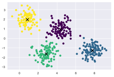
10.1 传统K-means聚类

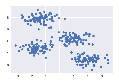
构造数据集

from sklearn.datasets.samples_generator importmake_blobs

X, y_true= make_blobs(n_samples=300, centers=4, cluster_std=0.60, random_state=0)

plt.scatter(X[:,0], X[:,1], s=50)

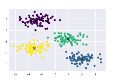
from sklearn.cluster importKMeans

kmeans= KMeans(n_clusters=4)

kmeans.fit(X)

y_kmeans= kmeans.predict(X)

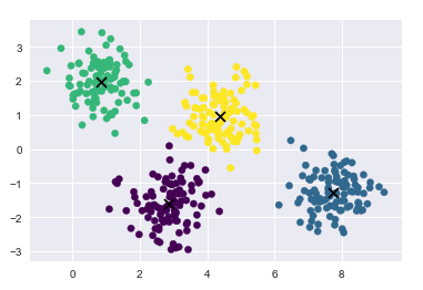
绘制聚类结果， 画出聚类中心

plt.scatter(X[:, 0], X[:, 1], c=y_kmeans, s=50, cmap=‘viridis‘)

centers=kmeans.cluster_centers_

plt.scatter(centers[:,0], centers[:,1], c=‘black‘, s=80, marker=‘x‘)

10.2 非线性边界聚类

对于非线性边界的kmeans聚类的介绍，查阅于《python数据科学手册》P410

构造数据

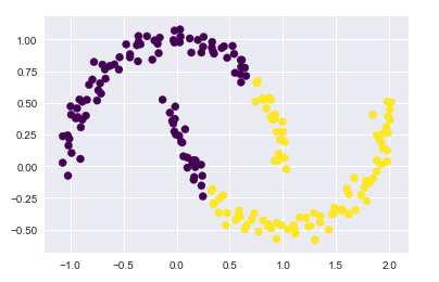
from sklearn.datasets importmake_moons

X, y= make_moons(200, noise=0.05, random_state=0)

传统kmeans聚类失败的情况

labels = KMeans(n_clusters=2, random_state=0).fit_predict(X)

plt.scatter(X[:, 0], X[:,1], c=labels, s=50, cmap=‘viridis‘)

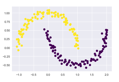
应用核方法， 将数据投影到更高纬的空间，变成线性可分

from sklearn.cluster importSpectralClustering

model= SpectralClustering(n_clusters=2, affinity=‘nearest_neighbors‘, assign_labels=‘kmeans‘)

labels=model.fit_predict(X)

plt.scatter(X[:, 0], X[:,1], c=labels, s=50, cmap=‘viridis‘)

10.3 预测结果与真实标签的匹配

手写数字识别例子

from sklearn.datasets importload_digits

digits= load_digits()

进行聚类

kmeans = KMeans(n_clusters=10, random_state=0)

clusters=kmeans.fit_predict(digits.data)

kmeans.cluster_centers_.shape

(10, 64)

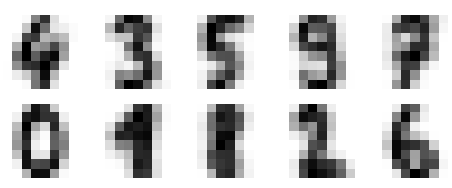
可以将这些族中心点看做是具有代表性的数字

fig, ax = plt.subplots(2, 5, figsize=(8, 3))

centers= kmeans.cluster_centers_.reshape(10, 8, 8)for axi, center inzip(ax.flat, centers):

axi.set(xticks=[], yticks=[])

axi.imshow(center, interpolation=‘nearest‘, cmap=plt.cm.binary)

进行众数匹配

from scipy.stats importmode

labels=np.zeros_like(clusters)for i in range(10):#得到聚类结果第i类的 True Flase 类型的index矩阵

mask = (clusters ==i)#根据index矩阵，找出这些target中的众数，作为真实的label

labels[mask] =mode(digits.target[mask])[0]#有了真实的指标，可以进行准确度计算

accuracy_score(digits.target, labels)0.7935447968836951

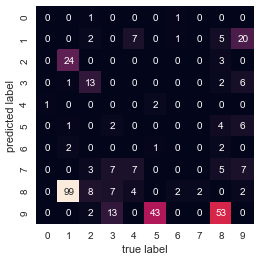
10.4 聚类结果的混淆矩阵

from sklearn.metrics importconfusion_matrix

mat=confusion_matrix(digits.target, labels)

np.fill_diagonal(mat, 0)

sns.heatmap(mat.T, square=True, annot=True, fmt=‘d‘, cbar=False,

xticklabels=digits.target_names,

yticklabels=digits.target_names)

plt.xlabel(‘true label‘)

plt.ylabel(‘predicted label‘)

10.5 t分布邻域嵌入预处理

即将高纬的 非线性的数据

通过流形学习

投影到低维空间

from sklearn.manifold importTSNE#投影数据#此过程比较耗时

tsen = TSNE(n_components=2, init=‘pca‘, random_state=0)

digits_proj=tsen.fit_transform(digits.data)#计算聚类的结果

kmeans = KMeans(n_clusters=10, random_state=0)

clusters=kmeans.fit_predict(digits_proj)#将聚类结果和真实标签进行匹配

labels =np.zeros_like(clusters)for i in range(10):

mask= (clusters ==i)

labels[mask]=mode(digits.target[mask])[0]#计算准确度

accuracy_score(digits.target, labels)

11. 高斯混合模型(聚类、密度估计)

k-means算法的非概率性和仅根据到族中心的距离指派族的特征导致该算法性能低下

且k-means算法只对简单的，分离性能好的，并且是圆形分布的数据有比较好的效果

本例中所有代码的实现已上传至 git仓库

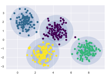
11.1 观察K-means算法的缺陷

通过实例来观察K-means算法的缺陷

%matplotlib inlineimportmatplotlib.pyplot as pltimportseaborn as sns; sns.set()importnumpy as np#生成数据点

from sklearn.datasets.samples_generator importmake_blobs

X, y_true= make_blobs(n_samples=400, centers=4,

cluster_std=0.60, random_state=0)

X= X[:, ::-1] #flip axes for better plotting#绘制出kmeans聚类后的标签的结果

from sklearn.cluster importKMeans

kmeans= KMeans(4, random_state=0)

labels=kmeans.fit(X).predict(X)

plt.scatter(X[:, 0], X[:,1], c=labels, s=40, cmap=‘viridis‘);

centers=kmeans.cluster_centers_

plt.scatter(centers[:,0], centers[:,1], c=‘black‘, s=80, marker=‘x‘)

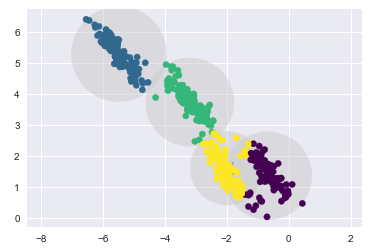
k-means算法相当于在每个族的中心放置了一个圆圈，(针对此处的二维数据来说)

半径是根据最远的点与族中心点的距离算出

下面用一个函数将这个聚类圆圈可视化

from sklearn.cluster importKMeansfrom scipy.spatial.distance importcdistdef plot_kmeans(kmeans, X, n_clusters=4, rseed=0, ax=None):

labels=kmeans.fit_predict(X)#plot the input data

ax = ax orplt.gca()

ax.axis(‘equal‘)

ax.scatter(X[:, 0], X[:,1], c=labels, s=40, cmap=‘viridis‘, zorder=2)#plot the representation of the KMeans model

centers=kmeans.cluster_centers_

ax.scatter(centers[:,0], centers[:,1], c=‘black‘, s=150, marker=‘x‘)

radii= [cdist(X[labels == i], [center]).max() for i, center inenumerate(centers)]#用列表推导式求出每一个聚类中心 i = 0, 1, 2, 3在自己的所属族的距离的最大值

#labels == i 返回一个布尔型index，所以X[labels == i]只取出i这个族类的数据点

#求出这些数据点到聚类中心的距离cdist(X[labels == i], [center]) 再求最大值 .max()

for c, r inzip(centers, radii):

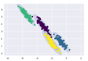
ax.add_patch(plt.Circle(c, r, fc=‘#CCCCCC‘, lw=3, alpha=0.5, zorder=1))#如果数据点不是圆形分布的

k-means算法的聚类效果就会变差

rng= np.random.RandomState(13)#这里乘以一个2,2的矩阵，相当于在空间上执行旋转拉伸操作

X_stretched = np.dot(X, rng.randn(2, 2))

kmeans= KMeans(n_clusters=4, random_state=0)

plot_kmeans(kmeans, X_stretched)

11.2 引出高斯混合模型

高斯混合模型能够计算出每个数据点，属于每个族中心的概率大小

在默认参数设置的、数据简单可分的情况下，

GMM的分类效果与k-means基本相同

from sklearn.mixture importGaussianMixture

gmm= GaussianMixture(n_components=4).fit(X)

labels=gmm.predict(X)

plt.scatter(X[:, 0], X[:,1], c=labels, s=40, cmap=‘viridis‘);#gmm的中心点叫做 means_

centers =gmm.means_

plt.scatter(centers[:,0], centers[:,1], c=‘black‘, s=80, marker=‘x‘);

得到数据的概率分布结果

probs =gmm.predict_proba(X)print(probs[:5].round(3))

[[0.0.469 0. 0.531]

[1. 0. 0. 0. ]

[1. 0. 0. 0. ]

[0. 0. 0.1. ]

[1. 0. 0. 0. ]]

编写绘制gmm绘制边界的函数

from matplotlib.patches importEllipsedef draw_ellipse(position, covariance, ax=None, **kwargs):"""Draw an ellipse with a given position and covariance"""ax= ax orplt.gca()#Convert covariance to principal axes

if covariance.shape == (2, 2):

U, s, Vt=np.linalg.svd(covariance)

angle= np.degrees(np.arctan2(U[1, 0], U[0, 0]))

width, height= 2 *np.sqrt(s)else:

angle=0

width, height= 2 *np.sqrt(covariance)#Draw the Ellipse

for nsig in range(1, 4):

ax.add_patch(Ellipse(position, nsig* width, nsig *height,

angle,**kwargs))def plot_gmm(gmm, X, label=True, ax=None):

ax= ax orplt.gca()

labels=gmm.fit(X).predict(X)iflabel:

ax.scatter(X[:, 0], X[:,1], c=labels, s=40, cmap=‘viridis‘, zorder=2)else:

ax.scatter(X[:, 0], X[:,1], s=40, zorder=2)

ax.axis(‘equal‘)

w_factor= 0.2 /gmm.weights_.max()for pos, covar, w inzip(gmm.means_, gmm.covariances_, gmm.weights_):

draw_ellipse(pos, covar, alpha=w * w_factor)

在圆形数据上的聚类结果

gmm = GaussianMixture(n_components=4, random_state=42)

plot_gmm(gmm, X)

在偏斜拉伸数据上的聚类结果

gmm = GaussianMixture(n_components=4, covariance_type=‘full‘, random_state=42)

plot_gmm(gmm, X_stretched)

11.3 将GMM用作密度估计

GMM本质上是一个密度估计算法；也就是说，从技术的角度考虑，

一个 GMM 拟合的结果并不是一个聚类模型，而是描述数据分布的生成概率模型。

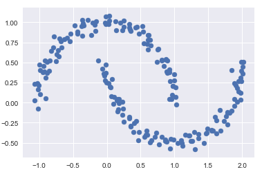
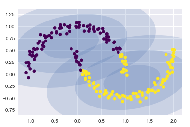
非线性边界的情况

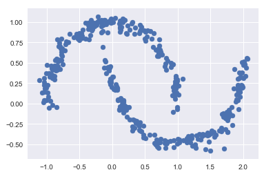
# 构建非线性可分数据

from sklearn.datasets importmake_moons

Xmoon, ymoon= make_moons(200, noise=.05, random_state=0)

plt.scatter(Xmoon[:, 0], Xmoon[:,1]);

? 如果使用2个成分聚类(即废了结果设置为2)，基本没什么效果

gmm2 = GaussianMixture(n_components=2, covariance_type=‘full‘, random_state=0)

plot_gmm(gmm2, Xmoon)

? 如果设置为多个聚类成分

gmm16 = GaussianMixture(n_components=16, covariance_type=‘full‘, random_state=0)

plot_gmm(gmm16, Xmoon, label=False)

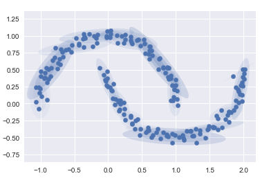
这里采用 16 个高斯曲线的混合形式不是为了找到数据的分隔的簇，而是为了对输入数据的总体分布建模。

11.4 由分布函数得到生成模型

分布函数的生成模型可以生成新的，与输入数据类似的随机分布函数(生成新的数据点)

用 GMM 拟合原始数据获得的 16 个成分生成的 400 个新数据点

Xnew = gmm16.sample(400)

Xnew[0][:5]

Xnew= gmm16.sample(400)

plt.scatter(Xnew[0][:, 0], Xnew[0][:,1]);

11.5 需要多少成分？

作为一种生成模型，GMM 提供了一种确定数据集最优成分数量的方法。

赤池信息量准则(Akaike information criterion) AIC

贝叶斯信息准则(Bayesian information criterion) BIC

n_components = np.arange(1, 21)

models= [GaussianMixture(n, covariance_type=‘full‘, random_state=0).fit(Xmoon)for n inn_components]

plt.plot(n_components, [m.bic(Xmoon)for m in models], label=‘BIC‘)

plt.plot(n_components, [m.aic(Xmoon)for m in models], label=‘AIC‘)

plt.legend(loc=‘best‘)

plt.xlabel(‘n_components‘);

观察可得，在 8~12 个主成分的时候，AIC 较小

评价指标

一、分类算法

常用指标选择方式

平衡分类问题：

分类准确度、ROC曲线

类别不平衡问题：

精准率、召回率

对于二分类问题，常用的指标是 f1 、 roc_auc

多分类问题，可用的指标为 f1_weighted

1.分类准确度

一般用于平衡分类问题(每个类比的可能性相同)

from sklearn.metrics importaccuracy_score

accuracy_score(y_test, y_predict)#(真值，预测值)

2. 混淆矩阵、精准率、召回率

精准率：正确预测为1 的数量，占，所有预测为1的比例

召回率：正确预测为1 的数量，占， 所有确实为1的比例

#先真实值，后预测值

from sklearn.metrics importconfusion_matrix

confusion_matrix(y_test, y_log_predict)from sklearn.metrics importprecision_score

precision_score(y_test, y_log_predict)from sklearn.metrics importrecall_score

recall_score(y_test, y_log_predict)

多分类问题中的混淆矩阵

多分类结果的精准率

from sklearn.metrics importprecision_score

precision_score(y_test, y_predict, average="micro")

多分类问题中的混淆矩阵

from sklearn.metrics importconfusion_matrix

confusion_matrix(y_test, y_predict)

移除对角线上分类正确的结果，可视化查看其它分类错误的情况

同样，横坐标为预测值，纵坐标为真实值

cfm =confusion_matrix(y_test, y_predict)

row_sums= np.sum(cfm, axis=1)

err_matrix= cfm /row_sums

np.fill_diagonal(err_matrix, 0)

plt.matshow(err_matrix, cmap=plt.cm.gray)

plt.show()

3.F1-score

F1-score是精准率precision和召回率recall的调和平均数

from sklearn.metrics importf1_score

f1_score(y_test, y_predict)

4.精准率和召回率的平衡

可以通过调整阈值，改变精确率和召回率(默认阈值为0)

拉高阈值，会提高精准率，降低召回率

降低阈值，会降低精准率，提高召回率

#返回模型算法预测得到的成绩#这里是以 逻辑回归算法 为例

decision_score =log_reg.decision_function(X_test)#调整阈值为5

y_predict_2 = np.array(decision_score >= 5, dtype=‘int‘)#返回的结果是0 、1

5.精准率-召回率曲线(PR曲线)

from sklearn.metrics importprecision_recall_curve

precisions, recalls, thresholds=precision_recall_curve(y_test, decision_score)#这里的decision_score是上面由模型对X_test预测得到的对象

绘制PR曲线

#精确率召回率曲线

plt.plot(precisions, recalls)

plt.show()

将精准率和召回率曲线，绘制在同一张图中

注意，当取“最大的” threshold值的时候，精准率=1，召回率=0，

但是，这个最大的threshold没有对应的值

因此thresholds会少一个

plt.plot(thresholds, precisions[:-1], color=‘r‘)

plt.plot(thresholds, recalls[:-1], color=‘b‘)

plt.show()

6.ROC曲线

Reciver Operation Characteristic Curve

TPR： True Positive rate

FPR： False Positive Rate

\[FPR=\frac{FP}{TN+FP} \]

绘制ROC曲线

from sklearn.metrics importroc_curve

fprs, tprs, thresholds=roc_curve(y_test, decision_scores)

plt.plot(fprs, tprs)

plt.show()

计算ROC曲线下方的面积的函数

roc_ area_ under_ curve_score

from sklearn.metrics importroc_auc_score

roc_auc_score(y_test, decision_scores)

曲线下方的面积可用于比较两个模型的好坏

总之，上面提到的decision_score 是一个概率值，如0 1 二分类问题，应该是将每个样本预测为1的概率，

如某个样本的y_test为1，y_predict_probablity为0.875

每个测试样本对应一个预测的概率值

通常在模型fit完成之后，都会有相应的得到概率的函数，如

model.predict_prob(X_test)

model.decision_function(X_test)

二、回归算法

1.均方误差 MSE

from sklearn.metrics importmean_squared_error

mean_squared_error(y_test, y_predict)

2.平均绝对值误差 MAE

from sklearn.metrics importmean_absolute_error

mean_absolute_error(y_test, y_predict)

3.均方根误差 RMSE

scikit中没有单独定于均方根误差，需要自己对均方误差MSE开平方根

4.R2评分

from sklearn.metrics importr2_score

r2_score(y_test, y_predict)

5.学习曲线

观察模型在训练数据集和测试数据集上的评分，随着训练数据集样本数增加的变化趋势。

importnumpy as npimportmatplot.pyplot as pltfrom sklearn.metrics importmean_squared_errordefplot_learning_curve(algo, X_train, X_test, y_train, y_test):

train_score=[]

test_score=[]for i in range(1, len(X_train)+1):

algo.fit(X_train[:i], y_train[:i])

y_train_predict=algo.predict(X_train[:i])

train_score.append(mean_squared_error(y_train[:i], y_train_predict))

y_test_predict=algo.predict(X_test)

test_score.append(mean_squared_error(y_test, y_test_predict))

plt.plot([ifor i in range(1, len(X_train)+1)], np.sqrt(train_score), label="train")

plt.plot([ifor i in range(1, len(X_train)+1)], np.sqrt(test_score), label="test")

plt.legend()

plt.axis([0,len(X_train)+1, 0, 4])

plt.show()#调用

plot_learning_curve(LinearRegression(), X_train, X_test, y_train, y_test )