【pytorch】手写数字分类全连接模型，并且出了正确率损失的效果图，逐行敲代码

---

前言

夯实基础系列，pytorch内置了很多全连接模型，我们可以用它来学习

---

1 前置

引入需要的库

import torch
import torch.nn as nn
import torch.nn.functional as F
import torch.optim as optim
import numpy as np
import matplotlib.pyplot as plt

1.1 torchvision 内置了常用数据集和常见模型

import torchvision
from torchvision import datasets, transforms
transformation = transforms.Compose([transforms.ToTensor()])

Compose 里面可以包很多数据增强的方式，随机裁剪，旋转之类的。但都会用到 ToTensor（）方法

1.2 数据集

train_ds = datasets.MNIST('data/',train=True,transform=transformation,download=True)
test_ds = datasets.MNIST('data/',train=False,transform=transformation,download=True)
train_dl = torch.utils.data.DataLoader(train_ds, batch_size=64,shuffle=True)
test_dl = torch.utils.data.DataLoader(test_ds,batch_size=256)

这里下载下来的图片是二进制打包格式的，其实很多Auto-ml 的平台也是这样做的，数据集散开比较费时间，时间都花在磁盘io上了，打包给比较好。

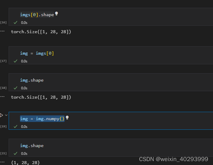
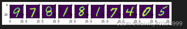
1.3 数据初探

imgs, labels = next(iter(train_dl))
imgs.shape
torch.Size([64, 1, 28, 28])

def imshow(img):
    npimg = img.numpy()
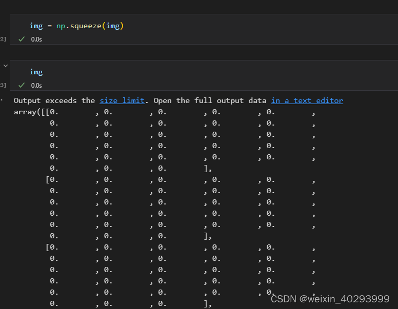
    npimg = np.squeeze(npimg)
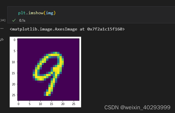
    plt.imshow(npimg)

plt.figure(figsize=(10,1))
for i, img in enumerate(imgs[:10]):
    plt.subplot(1,10,i+1)
    imshow(img)

2、模型构建&训练

2.1 模型构建

class Model(nn.Module):
    def __init__(self):
        super().__init__()
        self.linear_1 = nn.Linear(28*28,120)
        self.linear_2 = nn.Linear(120,84)
        self.linear_3 = nn.Linear(84,10)
    
    def forward(self, input):
        x = input.view(-1, 28*28)
        x = F.relu(self.linear_1(x))
        x = F.relu(self.linear_2(x))
        x = self.linear_3(x)
        return x
loss_fn = torch.nn.CrossEntropyLoss() # 损失函数

2.2 定义训练

model = Model()

def fit(epoch, model,trainloader, testloader):
    correct = 0 
    total = 0
    running_loss = 0
    for x, y in trainloader:
        y_pred = model(x)
        loss = loss_fn(y_pred, y)
        optim.zero_grad()
        loss.backward()
        optim.step()
        with torch.no_grad():
            y_pred = torch.argmax(y_pred,dim=1)
            correct += (y_pred == y).sum().item()
            total += y.size(0)
            running_loss += loss.item()
    
    epoch_loss = running_loss/len(trainloader.dataset)
    epoch_acc = correct/total

    test_correct = 0
    test_total = 0
    test_running_loss = 0
	with torch.no_grad():
        for x,y in testloader:
            y_pred = model(x)
            loss = loss_fn(y_pred, y)
            y_pred = torch.argmax(y_pred, dim=1)
            test_correct += (y_pred == y).sum().item()
            test_total += y.size(0)
            test_running_loss += loss.item()
    
    epoch_test_loss = test_running_loss / len(testloader.dataset)
    epoch_test_acc = test_correct / test_total

    print('epoch: ', epoch, 
        'loss： ', round(epoch_loss, 3),
        'accuracy:', round(epoch_acc, 3),
        'test_loss： ', round(epoch_test_loss, 3),
        'test_accuracy:', round(epoch_test_acc, 3)
            )
        
    return epoch_loss, epoch_acc, epoch_test_loss, epoch_test_acc

2.3 定义目标函数&训练

optim = torch.optim.Adam(model.parameters(), lr=0.001)
epochs = 20
train_loss = []
train_acc = []
test_loss = []
test_acc = []
for epoch in range(epochs):
    epoch_loss, epoch_acc, epoch_test_loss, epoch_test_acc = fit(epoch, model, train_dl, test_dl)

    train_loss.append(epoch_loss)
    train_acc.append(epoch_acc)
    test_loss.append(epoch_test_loss)
    test_acc.append(epoch_test_acc)

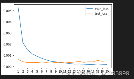
2.4 画图

import matplotlib.pyplot as plt
from matplotlib.pyplot import MultipleLocator
x_major_locator=MultipleLocator(1)
ax=plt.gca()
ax.xaxis.set_major_locator(x_major_locator)
plt.plot(range(1,epochs+1),train_loss,label="train_loss")
plt.plot(range(1,epochs+1),test_loss,label="test_loss")
plt.legend()

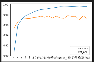
import matplotlib.pyplot as plt
x_major_locator=MultipleLocator(1)
ax=plt.gca()
ax.xaxis.set_major_locator(x_major_locator)
plt.plot(range(1,epochs+1),train_acc,label="train_acc")
plt.plot(range(1,epochs+1),test_acc,label="test_acc")
plt.legend()

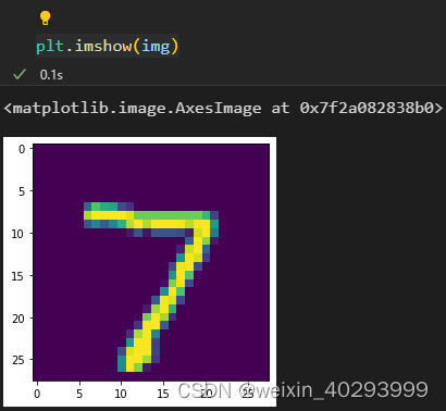
2.5 推理验证

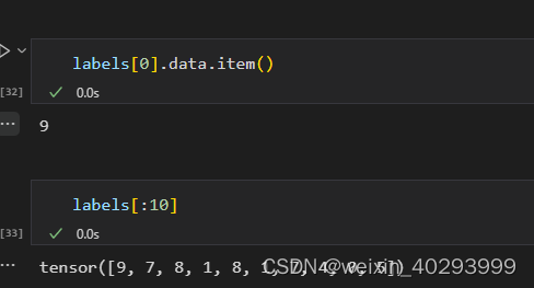
imgs, labels = next(iter(test_dl))
img = imgs[0]
label = labels[0]
img.shape
# torch.Size([28, 28])
# 模型肯定是[1,28,28] 需要增加一个bz纬度
img = np.squeeze(img)
y_pred = model(img)
y_pred = torch.argmax(y_pred, dim=1)
y_pred # 7

总结

这就是今天的全部知识了啊