PCA针对TE过程（田纳西伊斯曼过程）数据的故障监测处理

PCA故障诊断中两个关键统计变量$T^2$和$SPE$的的计算

$T^2$：Hotelling-T2
$SPE$：平方预测误差(Squared prediction error)

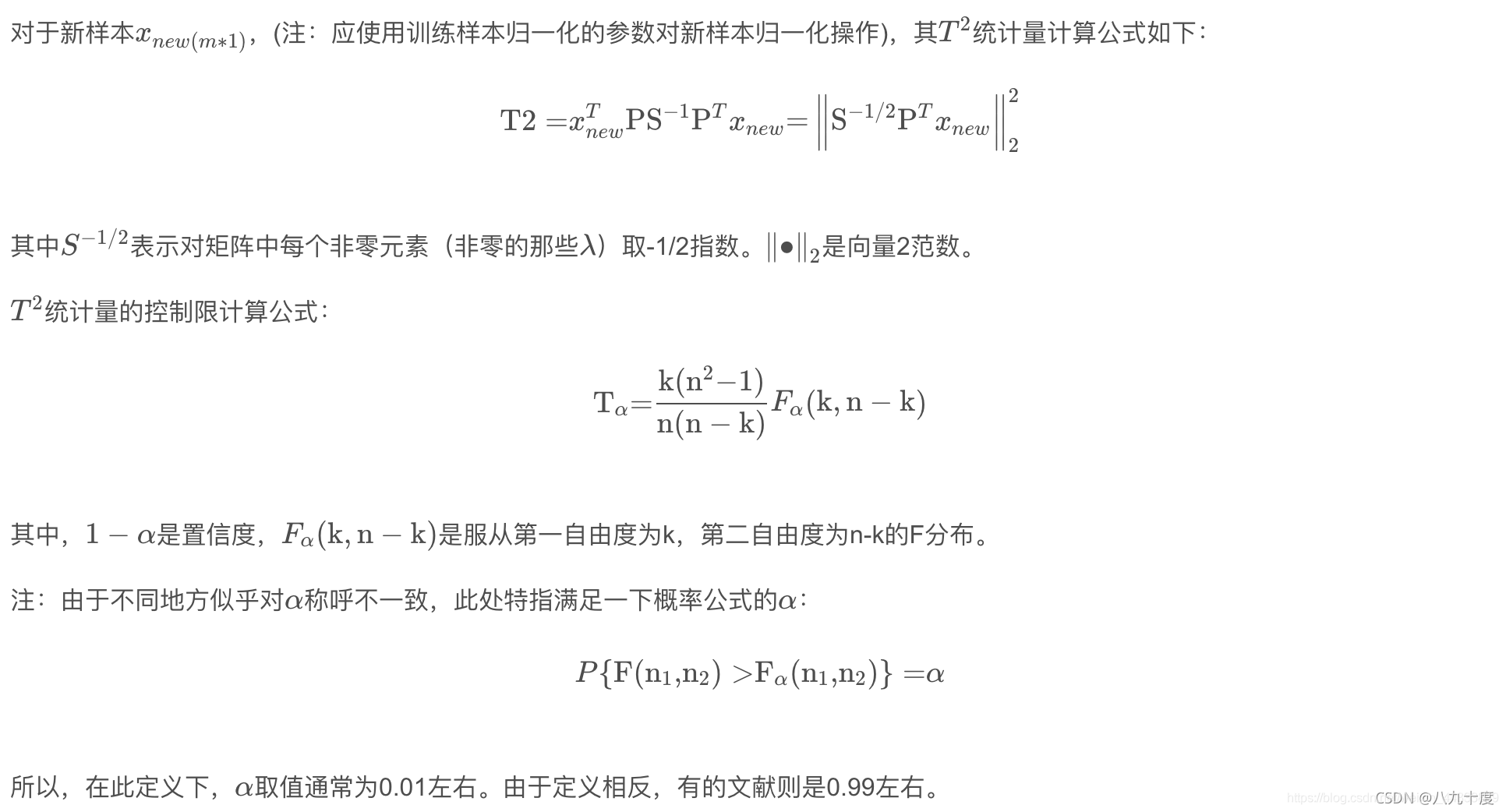
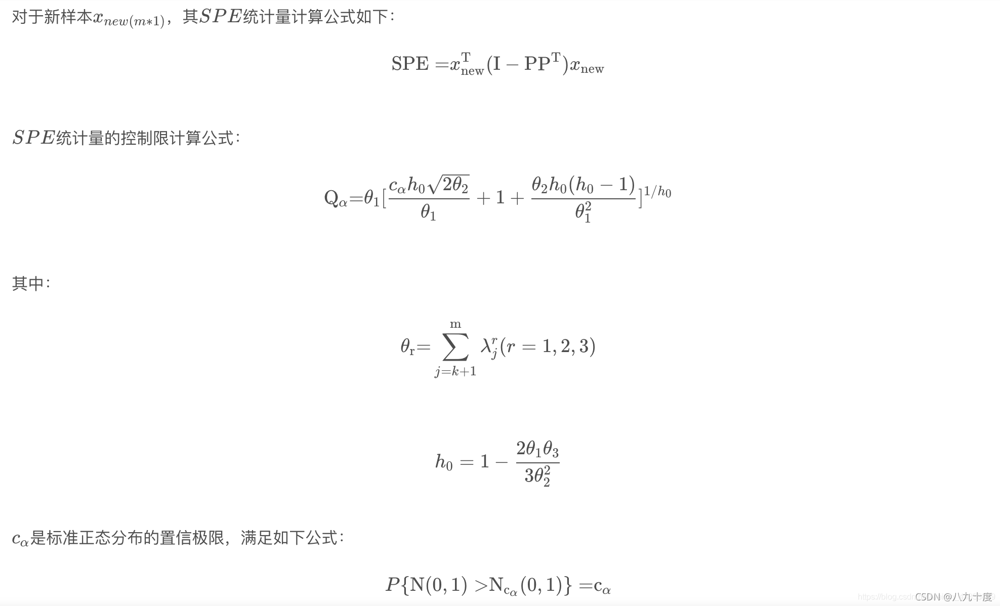
$T^2$ 统计量反映了每个主成分在变化趋势和幅值上偏离模型的程度，是对模型内部化的一种度量，它可以用来对多个主元同时进行监测；$SPE$ 统计量刻画了输入变量的测量值对主元模型的偏离程度，是对模型外部变化的一种度量。

$T^2$在线计算以及控制限的计算

$SPE$在线计算以及控制限的计算

$T^2$和$SPE$使用情况总结

• $T^2$统计量反应的是主元空间的变化，因此不能检测到非主元变量的故障；
• $SPE$统计量反应的是所有的变量，因此$T^2$统计量超限，$SPE$必超限（但有例外，如过程参数的变化）；
• 而$SPE$统计量衡量的是变量间相关性被改变的程度，显示异常的工况；所以当其超限时，可能是过程变量故障，也可能其它故障引起的。

根据$T^2$和$SPE$是否超限结果分析

1. 故障使$SPE$和$T^2$统计量同时超限；
2. 故障使$SPE$超限，而$T^2$统计量没有；
3. 故障使$T^2$ 统计量超限，而$SPE$没有；
4. 两者都没有超限。
   其中，$SPE$统计量对1,2,4是有效的。

两者的优缺点

$T^2$统计量适合来监控质量指标的变化；$SPE$统计量可以监控各类指标，其误报率和漏报率会少一些（针对非正态或者不平稳的过程）。

TE过程（田纳西伊斯曼过程）数据简介

具体数据见链接TE过程数据

在TE仿真平台中，可获取41个过程变量的运行数据和11个操纵变量的数据。另外，通过对进料等变量的输入控制，可以模拟得到21个故障类型，其中正常数据和异常（故障）数据的采样时间均为3min，即20次/min。
TE训练集和测试集结构：
整个TE数据集由训练集和测试集构成，TE集中的数据由22次不同的仿真运行数据构成，TE集中每个样本都有52个观测变量。d00.dat至d21.dat为训练集样本，d00_te.dat至d21_te.dat为测试集样本。前41个变量为过程变量，后11个变量为操纵变量。
d00.dat和d00_te.dat为正常工况下的样本。d00.dat训练样本是在25h运行仿真下获得的。观测数据总数为500。而d00_te.dat测试样本是在48h运行仿真下获得的，观测数据总数为960。
d01.dat至d21.dat为带有故障的训练集样本，d01_te.dat至d21_te.dat为带有故障的测试集样本。每个训练集\测试样本代表一种故障。
要值得注意的是对于带有故障的训练集样本，是在25h运行仿真下获得的。仿真开始时没有故障情况,故障是在仿真时间为1h的时候引入的。但观测数据是在引入故障后才开始采集的，即只有480个观测值。
带有故障的测试集样本是在48h运行仿真下获得的，故障在8h的时候引入，共采集960个观测值，其中前160个观测值为正常数据。

基于TE过程数据的PCA故障诊断

Python代码

read_TEdat.py：读取和处理TE过程原始.dat数据文件

import pandas as pd
import glob
import os
import matplotlib.pyplot as plt
plt.rcParams['font.sans-serif']=['SimHei'] #用来正常显示中文标签
plt.rcParams['axes.unicode_minus'] = False #用来正常显示负号

def read_all_data(path_test,path_train):
    '''
    读取TE过程的所有.dat数据并存人DataFrame中，输入参数为测试数据和训练数据的绝对路径
    '''
    var_name = []
    for i in range(1,42):
        var_name.append('XMEAS(' + str(i) + ')')
    for i in range(1,12):
        var_name.append('XMV(' + str(i) + ')')
    data_test, data_train = [], []
    # path_test = r'C:\Users\17253\Desktop\组内\K_shape\data\TE\test'
    # path_train = r'C:\Users\17253\Desktop\组内\K_shape\data\TE\train'
    test_join = glob.glob(os.path.join(path_test,'*.dat'))
    train_join = glob.glob(os.path.join(path_train,'*.dat'))
    for filename in test_join:
        data_test.append(pd.read_table(filename, sep = '\s+', header=None, engine='python', names = var_name))
    for filename2 in train_join:
        data_train.append(pd.read_table(filename2, sep = '\s+', header=None, engine='python', names = var_name))
    return data_test, data_train

diagnosis_pca.py：用PCA算法进行故障诊断

import numpy as np
import matplotlib.pyplot as plt
from sklearn.decomposition import PCA
from scipy import stats
from scipy.stats import norm, chi2
from sklearn.preprocessing import StandardScaler
plt.rcParams['font.sans-serif']=['SimHei'] #用来正常显示中文标签
plt.rcParams['axes.unicode_minus'] = False #用来正常显示负号


def t2_online(x, p, v):
    '''
    p：特征向量组成的降维矩阵，负载矩阵
    x：在线样本，shape为m*1
    v：特征值由大至小构成的对角矩阵
    '''
    T_2 = np.dot(np.dot((np.dot((np.dot(x.T, p)), np.linalg.inv(v))), p.T), x)
    return T_2

def spe_online(x, p):
    '''
    p：特征向量组成的降维矩阵，负载矩阵
    x：在线样本，shape为m*1
    '''
    I = np.eye(len(x))
    spe = np.dot(np.dot(x.T, I - np.dot(p, p.T)), x)
    # Q_count = np.linalg.norm(np.dot((I - np.dot(p_k, p_k.T)), test_data_nor), ord=None, axis=None, keepdims=False)  #二范数计算方法
    return spe

def pca_control_limit(Xtrain, ratio = 0.95, confidence = 0.99):
    '''
    计算出T2和SPE统计量
    '''
    pca = PCA(n_components = ratio)
    pca.fit(Xtrain)
    evr = pca.explained_variance_ratio_
    ev = pca.explained_variance_ # 方差，相当于X的协方差的最大的前几个特征值
    n_com = pca.n_components
    p = (pca.components_).T # 负载矩阵
    v = np.diag(ev) # 特征值组成的对角矩阵
    v_all = PCA(n_components = Xtrain.shape[1]).fit(Xtrain).explained_variance_
    p_all = (PCA(n_components = Xtrain.shape[1]).fit(Xtrain).components_).T
    k = len(evr)
    n_sample = pca.n_samples_
    ##T统计量阈值计算
    coe = k* (n_sample - 1) * (n_sample + 1) / ((n_sample - k) * n_sample)
    t_limit = coe * stats.f.ppf(confidence, k, (n_sample - k))

    ##SPE统计量阈值计算
    theta1 = np.sum((v_all[k:]) ** 1)
    theta2 = np.sum((v_all[k:]) ** 2)
    theta3 = np.sum((v_all[k:]) ** 3)
    h0 = 1 - (2 * theta1 * theta3) / (3 * (theta2 ** 2))
    c_alpha = norm.ppf(confidence)
    spe_limit = theta1 * ((h0 * c_alpha * ((2 * theta2) ** 0.5)
                           / theta1 + 1 + theta2 * h0 * (h0 - 1) / (theta1 ** 2)) ** (1 / h0))
    return t_limit, spe_limit, p, v, v_all, k, p_all

def pca_model_online(X, p, v):
    t_total = []
    q_total = []
    for x in range(np.shape(X)[0]):
        data_in = X[x]
        t = t2_online(data_in, p, v)
        q = spe_online(data_in, p)
        t_total.append(t)
        q_total.append(q)
    return t_total, q_total

def figure_control_limit(X, t_limit, spe_limit, t_total, q_total):
    ## 画控制限的图
    plt.figure(2, figsize=(12, 7))
    ax1 = plt.subplot(2, 1, 1)
    plt.plot(t_total)
    plt.plot(np.ones((len(X))) * t_limit, 'r', label='95% $T^2$ control limit')
    # ax1.set_ylim(0,100)
    # plt.xlim(0,100)
    ax1.set_xlabel(u'Samples')
    ax1.set_ylabel(u'Hotelling $T^2$ statistic')
    plt.legend()

    ax2 = plt.subplot(2, 1, 2)
    plt.plot(q_total)
    plt.plot(np.ones((len(X))) * spe_limit, 'r', label='95% spe control limit')
    # ax1.set_ylim(0,30)
    # plt.xlim(0,100)
    ax2.set_xlabel(u'Samples')
    ax2.set_ylabel(u'SPE statistic')
    plt.legend()
    plt.show()

def Contribution_graph(test_data, trian_data, index, p, p_all, v_all, k, t_limit):
    # 贡献图
    index = 160
    #1.确定造成失控状态的得分
    test_data = fault02_test
    data_mean = data_mean = np.mean(Xtrain_nor, 0)
    data_std = np.std(Xtrain_nor, 0)
    test_data_submean = np.array(test_data - data_mean)
    test_data_norm = np.array((test_data - data_mean) / data_std)
    t = test_data_norm[index,:].reshape(1,test_data.shape[1])
    S = np.dot(t,p[:,:])
    r = []
    for i in range(k):
        if S[0,i]**2/v_all[i] > t_limit/k:
            r.append(i)
    print(r)
    #2.计算每个变量相对于上述失控得分的贡献
    cont = np.zeros([len(r),test_data.shape[1]])
    for i in range(len(r)):
        for j in range(test_data.shape[1]):
            cont[i,j] = S[0,i]/v_all[r[i]]*p_all[r[i],j]*test_data_submean[index,j]
            if cont[i,j] < 0:
                cont[i,j] = 0
    #3.计算每个变量对T的总贡献
    a = cont.sum(axis = 0)
    #4.计算每个变量对Q的贡献
    I = np.eye(test_data.shape[1])
    e = (np.dot(test_data_norm[index,:],(I - np.dot(p, p.T))))**2

    ##画图
    plt.rcParams['font.sans-serif']=['SimHei']
    plt.rcParams['axes.unicode_minus'] = False
    font1 = {'family' : 'SimHei','weight' : 'normal','size'   : 23,}
    plt.figure(2,figsize=(16,9))
    ax1=plt.subplot(2,1,1)
    plt.bar(range(test_data.shape[1]),a)
    plt.xlabel(u'变量号',font1)
    plt.ylabel(u'T^2贡献率 %',font1)
    plt.legend()
    plt.show
    ax1=plt.subplot(2,1,2)
    plt.bar(range(test_data.shape[1]),e)
    plt.xlabel(u'变量号',font1)
    plt.ylabel(u'Q贡献率 %',font1)
    plt.legend()
    plt.show()

TE_mian：主函数

import read_TEdat
import diagnosis_pca as pca
from sklearn.preprocessing import StandardScaler
path_test = r'C:\Users\17253\Desktop\组内\K_shape\data\TE\test'
path_train = r'C:\Users\17253\Desktop\组内\K_shape\data\TE\train'
data_test, data_train = read_TEdat.read_all_data(path_test, path_train)
fault02_train, nor_train = data_train[2], data_train[0]
fault02_test, nor_test = data_test[2], data_test[0]

#数据标准化
scaler = StandardScaler().fit(nor_train)
Xtrain_nor = scaler.transform(nor_train)
Xtest_nor = scaler.transform(nor_test)
Xtrain_fault = scaler.transform(fault02_train)
Xtest_fault = scaler.transform(fault02_test)
# PCA
t_limit, spe_limit, p, v, v_all, k, p_all = pca.pca_control_limit(Xtrain_nor)

# 在线监测
t2, spe = pca.pca_model_online(Xtest_fault, p, v)

pca.figure_control_limit(Xtest_fault, t_limit, spe_limit, t2, spe)
pca.Contribution_graph(fault02_test, nor_train, 600, p, p_all, v_all, k, t_limit)
print(i)

结果分析

本次实验选择了故障2的数据作为测试数据d02_te.dat，训练数据使用训练集中的正常数据d00.dat。故障2的具体故障表现为组分B含量发生变化，A/C进料流量比不变（流4），类型为阶跃型。

$T^2$和$SPE$统计量监测

最后测试集的$T^2$和$SPE$统计量如图：

可以看出，在160个样本左右诊断出故障，与实际情况相符（具体的故障数据说明参考TE过程数据）

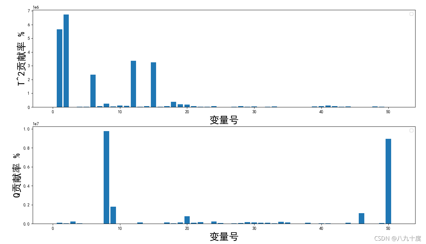
故障贡献图

一般变量的贡献越大，说明受其影响越大。
相关代码如下(diagnosis.Contribution_graph)：

def Contribution_graph(test_data, trian_data, index, p, p_all, v_all, k, t_limit):
    # 贡献图
    index = 160
    #1.确定造成失控状态的得分
    test_data = fault02_test
    data_mean = data_mean = np.mean(Xtrain_nor, 0)
    data_std = np.std(Xtrain_nor, 0)
    test_data_submean = np.array(test_data - data_mean)
    test_data_norm = np.array((test_data - data_mean) / data_std)
    t = test_data_norm[index,:].reshape(1,test_data.shape[1])
    S = np.dot(t,p[:,:])
    r = []
    for i in range(k):
        if S[0,i]**2/v_all[i] > t_limit/k:
            r.append(i)
    print(r)
    #2.计算每个变量相对于上述失控得分的贡献
    cont = np.zeros([len(r),test_data.shape[1]])
    for i in range(len(r)):
        for j in range(test_data.shape[1]):
            cont[i,j] = S[0,i]/v_all[r[i]]*p_all[r[i],j]*test_data_submean[index,j]
            if cont[i,j] < 0:
                cont[i,j] = 0
    #3.计算每个变量对T的总贡献
    a = cont.sum(axis = 0)
    #4.计算每个变量对Q的贡献
    I = np.eye(test_data.shape[1])
    e = (np.dot(test_data_norm[index,:],(I - np.dot(p, p.T))))**2

    ##画图
    plt.rcParams['font.sans-serif']=['SimHei']
    plt.rcParams['axes.unicode_minus'] = False
    font1 = {'family' : 'SimHei','weight' : 'normal','size'   : 23,}
    plt.figure(2,figsize=(16,9))
    ax1=plt.subplot(2,1,1)
    plt.bar(range(test_data.shape[1]),a)
    plt.xlabel(u'变量号',font1)
    plt.ylabel(u'T^2贡献率 %',font1)
    plt.legend()
    plt.show
    ax1=plt.subplot(2,1,2)
    plt.bar(range(test_data.shape[1]),e)
    plt.xlabel(u'变量号',font1)
    plt.ylabel(u'Q贡献率 %',font1)
    plt.legend()
    plt.show()

贡献图