CornerNet:Detecting Objects as Paired Keypoints

论文思想

将检测问题建模成关键点检测问题，通过检测左上、右下两个关键点来回归出检测框，是一种anchor free 的目标检测算法。主要解决了anchor based方法的两大问题：

1. anchor based方法分配gt的策略会很大程度的导致正负样本不平衡的请款
2. anchor boxes生成会引入大量的超参，训练比较难

模型架构

以640*640为输入data,总Flops达到707.76GFLOPs
各个模块占比情况

layer	hourglass backbone	tl_pool	br_pool	tl_heat	br_heat	tl_off	br_off	tl_emb	br_emb
Flops	51.745%	11.162%	11.162%	4.419%	4.419%	4.274%	4.274%	4.272%	4.272%

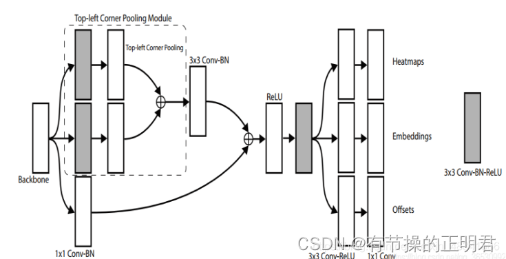
backbone

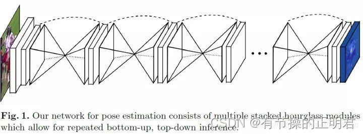
cornernet论文中backbone选择的是包含2个hourglasses的stacked hourglass网络，每个hourglasses中包含5次下采样和5次上采样过程，使用stride=2的3*3 conv替换maxpool以增强网络的学习能力。

输入data会经过stem layer(77 stride=2的conv+reslayer stride=2)将feature map降为（640/4）（6404），通道数变为256。之后经过hourglass module。
hourglass结构就是类似沙漏的网络结构，先经过5次下采样将160160256变为（160/32）（160/32）512，之后再通过5次上采样将55512恢复成160160*256。之所以设计这样的网络结构主要是为了捕获各个尺度下的信息，从而更适合关键点检测这种需要综合考虑局部和全局信息的任务。由于下采样、上采样过程中会产生信息损失，因此使用skip layer将下采样前的特征加回到上采样后的feature map中，减少信息损失。

intermediate supervision

传统的识别或者检测网络，loss只比较最后的预测与ground truth之间的差异。因为堆叠沙漏网络的每一个子沙漏网络都会有heat map作为预测，所以将每个沙漏输出的heat map参与到loss中，实验证实，预测精确度要远远好于只考虑最后一个沙漏预测的loss，这种考虑网络中间部分的监督训练方式，就叫做中间监督。

tl_pool br_pool

cornernet中提出了corner pool的概念。object的角点通常来说都是没有语义信息的，为了更好的定位角点，提出使用corner pool来解决。
对于左上角点来说，为了更好的定位左上角点，需要对从左至右的特征和由上至下的“优势”特征进行特征增强。
具体做法：首先需要由backbone输出的featuremap x分别得到垂直方向、竖直方向特征图，命名为ft fl。

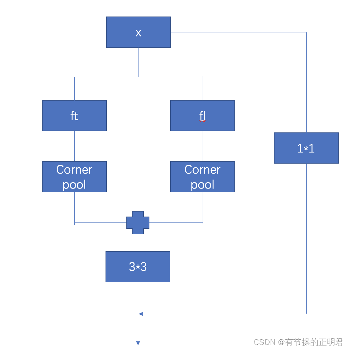
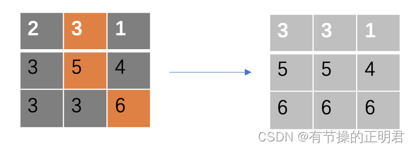
corner pool的过程比较简单，简单来说就是使用maxpool实现优势特征点在对应方向上的延续，以增强左上角特征。
例如ft为

fl

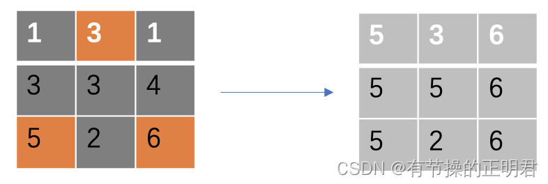
将经过corner pool后的ft和fl相加即可得到tl经过corner pool后的特征

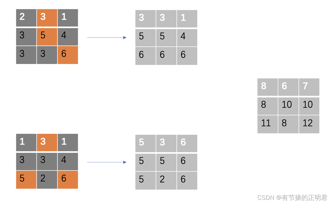
也就是尽可能将大元素集中在feature map的左上部分。论文里实验表明，通过加入cornermap，tl、br的map都有3个点左右的提升。
后面得到tl heat map 、tl offset、tl emb等feature map都是基于cornermap之后的特征图

如何匹配角点

corner match怎么做也是这篇论文中一个关键点。tl heat map brheatmap确实可以得到所有可能的左上、右下角点，但是哪个左上、右下同属于一个检测框却不得而知。此篇论文的策略是分别预测tl和br的embedding，让同属于一个检测框的embedding值尽可能相近，不同检测框的embedding差值尽可能大。这样在预测时只需要比较tl br embedding的L1距离即可将corner匹配上。

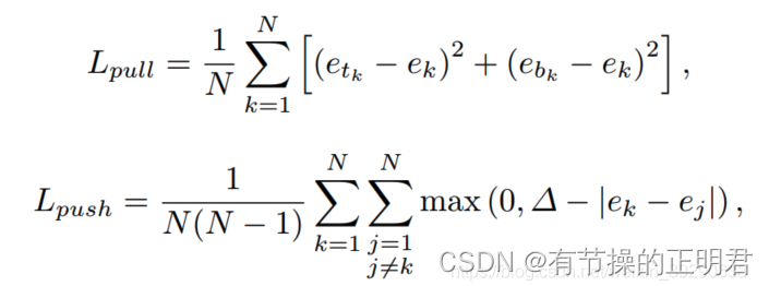
embedding loss设计

embeddding的具体值对于网络来说并不重要，主要原则是同属一个框的tl br的embedding距离要足够近，不同框之间的tl br的embedding距离要足够远。因此设计了Lpull 和Lpush来共同计算embedding的loss

具体实现

def ae_loss_per_image(tl_preds, br_preds, match):
    """Associative Embedding Loss in one image.

    Associative Embedding Loss including two parts: pull loss and push loss.
    Pull loss makes embedding vectors from same object closer to each other.
    Push loss distinguish embedding vector from different objects, and makes
        the gap between them is large enough.

    During computing, usually there are 3 cases:
        - no object in image: both pull loss and push loss will be 0.
        - one object in image: push loss will be 0 and pull loss is computed
            by the two corner of the only object.
        - more than one objects in image: pull loss is computed by corner pairs
            from each object, push loss is computed by each object with all
            other objects. We use confusion matrix with 0 in diagonal to
            compute the push loss.

    Args:
        tl_preds (tensor): Embedding feature map of left-top corner.
        br_preds (tensor): Embedding feature map of bottim-right corner.
        match (list): Downsampled coordinates pair of each ground truth box.
    """

    tl_list, br_list, me_list = [], [], []
    if len(match) == 0:  # no object in image
        pull_loss = tl_preds.sum() * 0.
        push_loss = tl_preds.sum() * 0.
    else:
        for m in match:
            [tl_y, tl_x], [br_y, br_x] = m
            tl_e = tl_preds[:, tl_y, tl_x].view(-1, 1)
            br_e = br_preds[:, br_y, br_x].view(-1, 1)
            tl_list.append(tl_e)
            br_list.append(br_e)
            me_list.append((tl_e + br_e) / 2.0)

        tl_list = torch.cat(tl_list)
        br_list = torch.cat(br_list)
        me_list = torch.cat(me_list)

        assert tl_list.size() == br_list.size()

        # N is object number in image, M is dimension of embedding vector
        N, M = tl_list.size()

        pull_loss = (tl_list - me_list).pow(2) + (br_list - me_list).pow(2)
        pull_loss = pull_loss.sum() / N

        margin = 1  # exp setting of CornerNet, details in section 3.3 of paper

        # confusion matrix of push loss
        conf_mat = me_list.expand((N, N, M)).permute(1, 0, 2) - me_list
        conf_weight = 1 - torch.eye(N).type_as(me_list)
        conf_mat = conf_weight * (margin - conf_mat.sum(-1).abs())

        if N > 1:  # more than one object in current image
            push_loss = F.relu(conf_mat).sum() / (N * (N - 1))
        else:
            push_loss = tl_preds.sum() * 0.

    return pull_loss, push_loss