


论文标题:See Better Before Looking Closer: Weakly Supervised Data AugmentationNetwork for Fine-Grained Visual Classification
针对目标:细粒度图像分类
下载地址:https://arxiv.org/pdf/1901.09891v2.pdf官方github地址: https://github.com/tau-yihouxiang/WS_DAN
pytorch复现版github地址:
本文看点
- 双线性注意力池化 (Bilinear Attention Pooling)
- 注意力正则化 (Attention Regularization)
- 注意力引导数据增强 (Attention-guided Data Augmentation)
- 测试阶段测试集的目标定位与图像精修.(Object Localization and Refinement)
1.双线性注意力池化
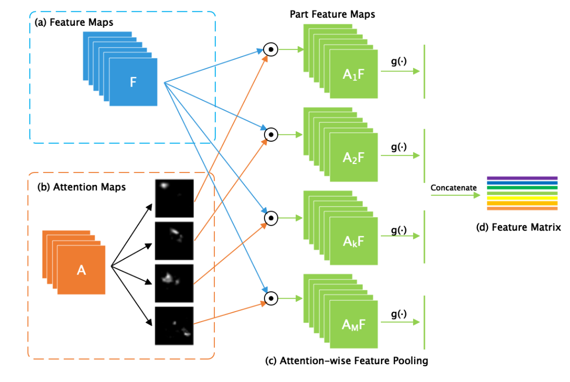
以inceptionv3作为backbone为例,取Mix6e层的输出为上图中的 (a)Feature Maps, 再对 (a) 进行 1 x 1 的卷积操作得到 (b)Attention Maps。
所谓的双线性注意力池化其实就是以 (b)Attention Maps作为指导,对 (a)Feature Maps中每个元素重新赋值得到( c), 我们可以用空间注意力机制的思想去理解。然后再进行池化与向量化操作得到(d)。
以上图为例,(b)Attention Maps有四个通道的注意力图,(a)Feature Maps有六个通道的特征图.那么每个注意力图都会分别与所有特征图进行元素相乘,得到四组特征图,每组特征图有6通道。进一步,将每组特征图进行最大池化并且向量化得到四组向量,然后四组向量拼接为一个特征矩阵。按照这种思想,上图中的 (d) 其实应该是画错了,理论上应该为四条向量,而作者画成了七条,不知我是否理解有误。
代码实现:
class BAP(nn.Module):
    def __init__(self,  **kwargs):
        super(BAP, self).__init__()
    def forward(self,feature_maps,attention_maps):
        feature_shape = feature_maps.size() ## 12*768*26*26
        attention_shape = attention_maps.size() ## 12*32*26*26
        phi_I = torch.einsum('imjk,injk->imn', (attention_maps, feature_maps)) ## 12*32*768
        phi_I = torch.div(phi_I, float(attention_shape[2] * attention_shape[3]))
        # 为什么还要对应元素相乘,第一个符号函数,第二个绝对值之后开根,文中未提及
        phi_I = torch.mul(torch.sign(phi_I), torch.sqrt(torch.abs(phi_I) + 1e-12))
        # 实际上没有去实现(d)的征矩阵,而是直接用一维特征向量替换,不过原理一样.
        phi_I = phi_I.view(feature_shape[0],-1)
        raw_features = torch.nn.functional.normalize(phi_I, dim=-1) ##12*(32*768)
        pooling_features = raw_features*100
        return raw_features,pooling_features
2.注意力正则化
为了让同一个类别中的同一个通道的注意力图专注于特定的区域,假定类别一的第一个通道的注意力图只专注于嘴部,作者提出了注意力正则化的方法.
以下,是两个通道可视化结果(第一行通道专注于脖子,第二行专注于嘴部)

以类别数,特征图数和注意力通道数为标准,设置一个特征中心
c
k
c_k
ck .以CUB数据集为例,200类别,设置32个注意力图,768个特征图,那么特征中心的维度为(200,32,768)。特征中心初始情况下所有元素都为0。以下面公式中滑动平均的方式来更新
c
k
c_k
ck,
β
β
β设置为0.05,
f
k
f_k
fk为(d)特征矩阵。通过不断的更新迭代,最终
c
k
c_k
ck趋于稳定。
c
k
←
c
k
+
β
(
f
k
−
c
k
)
c_{k} \leftarrow c_{k}+\beta\left(f_{k}-c_{k}\right)
ck←ck+β(fk−ck)
同时,设置损失函数用于指导更新
f
k
f_k
fk。
L
A
=
∑
k
=
1
M
∥
f
k
−
c
k
∥
2
2
L_{A}=\sum_{k=1}^{M}\left\|f_{k}-c_{k}\right\|_{2}^{2}
LA=k=1∑M∥fk−ck∥22
代码实现
def calculate_pooling_center_loss(features, centers, label, beta=0.05):
    features = features.reshape(features.shape[0], -1)
    centers_batch = centers[label]
    centers_batch = torch.nn.functional.normalize(centers_batch, dim=-1)
    diff =  beta*(features.detach() - centers_batch)
    distance = torch.pow(features - centers_batch,2)
    distance = torch.sum(distance, dim=-1)
    center_loss = torch.mean(distance)
    return center_loss, diff
3.注意力引导数据增强
作者提出了基于注意力的图像裁剪和图像擦除。
图像擦除: 在32个注意力图中,按照每个注意力图自身的均值与所有注意力图自身均值之和的比值作为抽样概率,选取出来一个注意力图。将该注意力图二值化,作为二进制掩码,与原图相乘,就遮挡住了一块判别性区域。
图像裁剪: 和上面类似,挑出一个注意力图,然后根据二进制掩码,找到一个包住二进制掩码中mask区域的最小的矩形框,用该矩形框裁剪原图,然后放大到原图大小。
代码实现
def attention_crop_drop2(attention_maps,input_image):
    B,N,W,H = input_image.shape
    input_tensor = input_image
    batch_size, num_parts, height, width = attention_maps.shape
    attention_maps = torch.nn.functional.interpolate(attention_maps.detach(),size=(W,H),mode='bilinear',align_corners=True)
    part_weights = F.avg_pool2d(attention_maps.detach(),(W,H)).reshape(batch_size,-1)
    part_weights = torch.add(torch.sqrt(part_weights),1e-12)
    part_weights = torch.div(part_weights,torch.sum(part_weights,dim=1).unsqueeze(1)).cpu()
    part_weights = part_weights.numpy()
    ret_imgs = []
    masks = []
    for i in range(batch_size):
        attention_map = attention_maps[i]
        part_weight = part_weights[i]
        selected_index = np.random.choice(np.arange(0, num_parts), 1, p=part_weight)[0]
        selected_index2 = np.random.choice(np.arange(0, num_parts), 1, p=part_weight)[0]
        ## create crop imgs
        mask = attention_map[selected_index, :, :]
        threshold = random.uniform(0.4, 0.6)
        itemindex = torch.nonzero(mask >= threshold*mask.max())
        padding_h = int(0.1*H)
        padding_w = int(0.1*W)
        height_min = itemindex[:,0].min()
        height_min = max(0,height_min-padding_h)
        height_max = itemindex[:,0].max() + padding_h
        width_min = itemindex[:,1].min()
        width_min = max(0,width_min-padding_w)
        width_max = itemindex[:,1].max() + padding_w
        out_img = input_tensor[i][:,height_min:height_max,width_min:width_max].unsqueeze(0)
        out_img = torch.nn.functional.interpolate(out_img,size=(W,H),mode='bilinear',align_corners=True)
        out_img = out_img.squeeze(0)
        ret_imgs.append(out_img)

        ## create drop imgs
        mask2 = attention_map[selected_index2:selected_index2 + 1, :, :]
        threshold = random.uniform(0.2, 0.5)
        mask2 = (mask2 < threshold * mask2.max()).float()
        masks.append(mask2)
    crop_imgs = torch.stack(ret_imgs)
    masks = torch.stack(masks)
    drop_imgs = input_tensor*masks
    return (crop_imgs,drop_imgs)
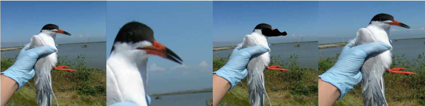
下图是我在复现论文时得到的可视化结果,从左到右为: 原图 -> 图像裁剪 -> 图像擦除->目标区域裁剪(测试阶段的裁剪方法)。
训练阶段的网络结构:
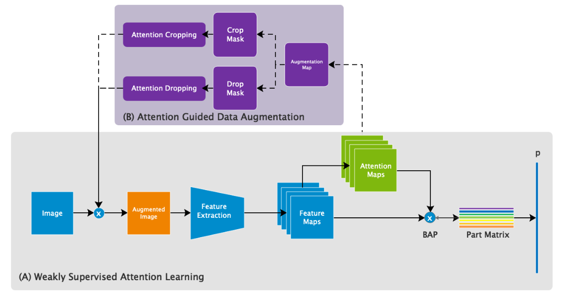
根据网络结构可知,先将原始图像送入网络训练,然后结合获取到的特征图与注意力图,对原图进行裁剪和丢弃操作,再将处理后的图片也送入网络训练。
4.测试阶段测试集的目标定位与图像精修
这一步是在测试阶段进行的,和注意力引导数据增强中的图像裁剪实现过程类似,不过这次是用到了所有的注意力图.通过对所有注意力图求平均,得到一张注意力图,然后定位到目标整体的位置,再将其裁剪放大,预测结果.
代码实现
def mask2bbox(attention_maps,input_image):
    input_tensor = input_image
    B,C,H,W = input_tensor.shape
    batch_size, num_parts, Hh, Ww = attention_maps.shape
    attention_maps = torch.nn.functional.interpolate(attention_maps,size=(W,H),mode='bilinear',align_corners=True)
    ret_imgs = []
    for i in range(batch_size):
        attention_map = attention_maps[i]
        mask = attention_map.mean(dim=0)
        threshold = 0.1
        max_activate = mask.max()
        min_activate = threshold * max_activate
        itemindex = torch.nonzero(mask >= min_activate)
        print(itemindex.shape)
        padding_h = int(0.05*H)
        padding_w = int(0.05*W)
        # 找到非零元素出现时最小的行数,并且将抠出的图放大一定范围
        height_min = itemindex[:, 0].min()
        height_min = max(0,height_min-padding_h)
        height_max = itemindex[:, 0].max() + padding_h
        width_min = itemindex[:, 1].min()
        width_min = max(0,width_min-padding_w)
        width_max = itemindex[:, 1].max() + padding_w
        out_img = input_tensor[i][:,height_min:height_max,width_min:width_max].unsqueeze(0)
        out_img = torch.nn.functional.interpolate(out_img,size=(W,H),mode='bilinear',align_corners=True)
        out_img = out_img.squeeze(0)
        ret_imgs.append(out_img)
    ret_imgs = torch.stack(ret_imgs)
    return ret_imgs
测试阶段的网络结构:
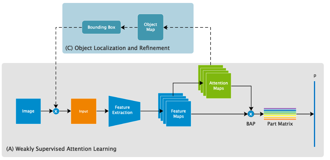
根据网络结构可知,先将原始图像送入网络预测结果,然后结合特征图与注意力图,对原图的目标区域进行裁剪,再将处理后的图片也送入网络预测,结合两次预测的结果,得到最终的预测输出。
实验结果
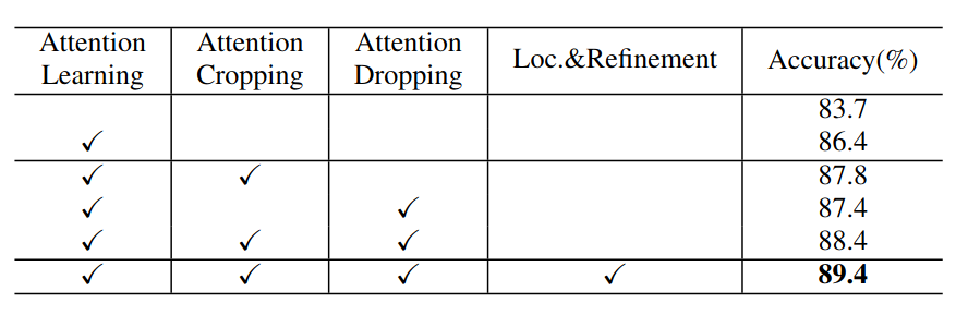
1.各个组件的贡献(CUB数据集)
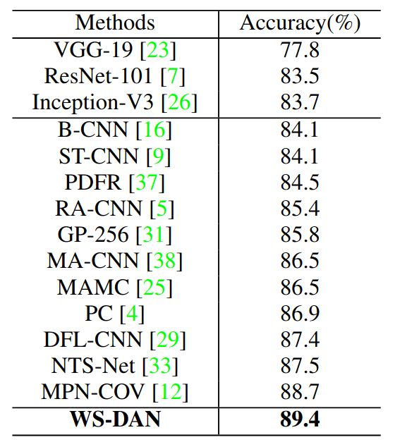
2.与SOTA比较(CUB数据集)


 3106
3106

 被折叠的 条评论
为什么被折叠?
被折叠的 条评论
为什么被折叠?
 到【灌水乐园】发言


