


反向传播算法实例
算例情景:
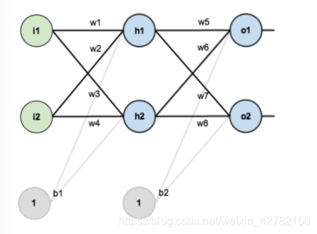
假设有一个如下图所示的三层结构的神经网络。其中,第一层是输入层,包含两个神经元
i
1
,
i
2
i_1, i_2
i1,i2 和截距项
b
1
b_1
b1 ;第二层是隐藏层,包含两个神经元
h
1
,
h
2
h_1, h_2
h1,h2 和截距项
b
2
b_2
b2 ;第三层是输出层,包含两个输出项
o
1
,
o
2
o_1, o_2
o1,o2。每条线上标的
w
i
w_i
wi表示层与层之间连接的权重,在本算例中激活函数默认选择
S
i
g
m
o
i
d
Sigmoid
Sigmoid函数。
接下来,对上面的神经网络模型赋初值,所得结果如下图所示:
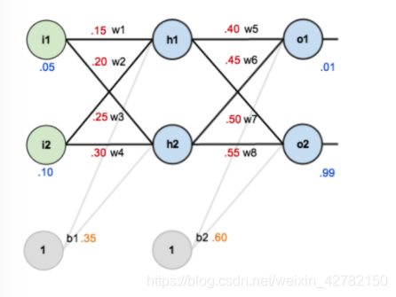
赋初值的具体取值情形如下,其中:
输入数据(原始输入):
i
1
=
0.05
,
i
2
=
0.10
;
i_1=0.05, i_2=0.10;
i1=0.05,i2=0.10;
输出数据(期望输出):
o
1
=
0.01
,
o
2
=
0.99
;
o_1=0.01, o_2=0.99;
o1=0.01,o2=0.99;
初始权重:
w
1
=
0.15
,
w
2
=
0.20
,
w
3
=
0.25
,
w
4
=
0.30
;
w_1=0.15, w_2=0.20, w_3=0.25, w_4=0.30;
w1=0.15,w2=0.20,w3=0.25,w4=0.30;
w
5
=
0.40
,
w
6
=
0.45
,
w
7
=
0.50
,
w
8
=
0.55
;
\quad \quad \quad \quad w_5=0.40, w_6=0.45, w_7=0.50, w_8=0.55;
w5=0.40,w6=0.45,w7=0.50,w8=0.55;
截距项:
b
1
=
0.35
,
b
2
=
0.60
;
b_1=0.35, b_2=0.60;
b1=0.35,b2=0.60;
预期目标: 根据给定的输入数据 i 1 , i 2 ( 0.05 和 0.10 ) i_1, i_2(0.05和0.10) i1,i2(0.05和0.10),通过反向传播算法进行“权值修正”,使得实际输出与期望输出 o 1 , o 2 ( 0.01 和 0.99 ) o_1, o_2(0.01和0.99) o1,o2(0.01和0.99)最接近(即:实际输出与期望输出之间误差最小)。
算法的基本原理:
算法实现过程主要分两步:
(1)前向传播: 求得初始状态下,实际输出和期望输出之间的总误差
Δ
0
Δ_0
Δ0;
(2)反向传播: 根据 “链式求导法则” 对输出层、隐藏层的权值进行修正,从而缩小实际输出与期望输出之间的总误差。
算法的求解过程:
Step1 前向传播
1. 输入层----> 隐藏层:
由从神经网络第 l − 1 l-1 l−1层的第 k k k个节点到神经网络第 l l l层的第 j j j个节点的输出结果的计算公式: z j l = ∑ k w j k l a k l − 1 + b j l z_j^l=\sum_kw_{jk}^la_k^{l-1}+b_j^l zjl=∑kwjklakl−1+bjl 可知:
本算例中,神经元
h
1
h_1
h1的输入加权和
n
e
t
h
1
net_{h_1}
neth1的计算如下:
n
e
t
h
1
=
w
1
∗
i
1
+
w
2
∗
i
2
+
b
1
∗
1
=
0.15
∗
0.05
+
0.2
∗
0.1
+
0.35
∗
1
=
0.3775
\begin{aligned} net_{h_1}&=w_1*i_1+w_2*i_2+b_1*1\\ &=0.15*0.05+0.2*0.1+0.35*1\\ &=0.3775 \end{aligned}
neth1=w1∗i1+w2∗i2+b1∗1=0.15∗0.05+0.2∗0.1+0.35∗1=0.3775
引入激活函数Sigmoid,计算神经元
h
1
h_1
h1的输出
o
u
t
h
1
out_{h_1}
outh1:
o
u
t
h
1
=
1
1
+
e
−
n
e
t
h
1
=
1
1
+
e
−
0.3775
=
0.59327
\begin{aligned} out_{h_1}&=\frac{1}{1+e^{-net_{h_1}}}\\ &=\frac{1}{1+e^{-0.3775}}\\ &=0.59327 \end{aligned}
outh1=1+e−neth11=1+e−0.37751=0.59327
同理,可以计算出神经元
h
2
h_2
h2的输出
o
u
t
h
2
out_{h_2}
outh2为:
o
u
t
h
2
=
0.59688
out_{h_2}=0.59688
outh2=0.59688
2. 隐藏层----> 输出层:
依次计算输出层神经元
o
1
o_1
o1和
o
2
o_2
o2的实际输出值,方法同上:
n
e
t
o
1
=
w
5
∗
o
u
t
h
1
+
w
6
∗
o
u
t
h
2
+
b
2
∗
1
=
0.40
∗
0.59327
+
0.45
∗
0.59688
+
0.60
∗
1
=
1.105904
\begin{aligned} net_{o_1}&=w_5*out_{h_1}+w_6*out_{h_2}+b_2*1\\ &=0.40*0.59327+0.45*0.59688+0.60*1\\ &=1.105904 \end{aligned}
neto1=w5∗outh1+w6∗outh2+b2∗1=0.40∗0.59327+0.45∗0.59688+0.60∗1=1.105904
引入激活函数Sigmoid,计算神经元
o
1
o_1
o1的输出
o
u
t
o
1
out_{o_1}
outo1:
o
u
t
o
1
=
1
1
+
e
−
n
e
t
o
1
=
1
1
+
e
−
1.105904
=
0.75136
\begin{aligned} out_{o_1}&=\frac{1}{1+e^{-net_{o_1}}}\\ &=\frac{1}{1+e^{-1.105904}}\\ &=0.75136 \end{aligned}
outo1=1+e−neto11=1+e−1.1059041=0.75136
同理可以计算神经元
o
2
o_2
o2的输出
o
u
t
o
2
out_{o_2}
outo2为:
o
u
t
o
2
=
0.772928
out_{o_2}=0.772928
outo2=0.772928
至此,通过前向传播计算神经网络实际输出的过程就结束了。最终求得实际输出值为
[
0.75136
,
0.772928
]
[0.75136, 0.772928]
[0.75136,0.772928],与期望输出
[
0.01
,
0.99
]
[0.01,0.99]
[0.01,0.99]还相差甚远。因此,接下来需要我们通过误差反向传播算法来更新权值,重新计算输出,以缩小实际输出与期望输出之间的总误差。
Step2 反向传播
1. 计算总误差:
本算例,引入均方根误差(MSE)求解实际输出与期望输出之间的总误差,计算公式为:
E t o t a l = ∑ i = 1 n 1 2 ( t a r g e t − o u t p u t ) 2 E_{total}=\sum_{i=1}^n \frac{1}{2}(target-output)^2 Etotal=i=1∑n21(target−output)2
备注: n n n表示输出神经元的个数, t a r g e t target target表示期望输出, o u t p u t output output表示实际输出。
在本算例中,神经网络有两个输出神经元,故
n
=
2
n=2
n=2,总误差即为两者之和:
E
o
1
=
1
2
(
t
a
r
g
e
t
o
1
−
o
u
t
o
1
)
2
=
1
2
(
0.01
−
0.75136
)
2
=
0.2748
\begin{aligned} E_{o_1}&=\frac{1}{2}(target_{o_1}-out_{o_1})^2\\ &=\frac{1}{2}(0.01-0.75136)^2\\ &=0.2748 \end{aligned}
Eo1=21(targeto1−outo1)2=21(0.01−0.75136)2=0.2748
同理,可以计算
E
o
2
E_{o_2}
Eo2的值为:
E
o
2
=
0.02356
E_{o_2}=0.02356
Eo2=0.02356
2. 输出层----> 隐藏层的权值更新:
核心思想: 对于整个神经网络的总误差 E t o t a l E_{total} Etotal,通过 “链式求导法则” 依次对各权重 w i w_i wi求偏导,从而得知权重 w i w_i wi对总误差产生了多少影响。
以总误差
E
t
o
t
a
l
E_{total}
Etotal对权重
w
5
w_5
w5的偏导过程为例,其误差的反向传播过程如图所示:
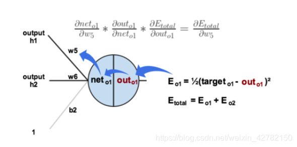
根据“链式求导法则”,计算公式为:
∂
E
t
o
t
a
l
∂
w
5
=
E
t
o
t
a
l
∂
o
u
t
o
1
∗
∂
o
u
t
o
1
∂
n
e
t
o
1
∗
∂
n
e
t
o
1
∂
w
5
\frac{\partial E_{total}}{\partial w_5}=\frac{E_{total}}{\partial{out_{o_1}}}*\frac{\partial{out_{o_1}}}{\partial net_{o_1}}*\frac{{\partial{net_{o_1}}}}{\partial w_5}
∂w5∂Etotal=∂outo1Etotal∗∂neto1∂outo1∗∂w5∂neto1
接下来,分别计算每个偏导分式的值:
(1)计算 E t o t a l ∂ o u t o 1 \frac{E_{total}}{\partial{out_{o_1}}} ∂outo1Etotal的值:
E
t
o
t
a
l
=
1
2
(
t
a
r
g
e
t
o
1
−
o
u
t
o
1
)
2
+
1
2
(
t
a
r
g
e
t
o
2
−
o
u
t
o
2
)
2
E_{total}=\frac{1}{2}(target_{o_1}-out_{o_1})^2+\frac{1}{2}(target_{o_2}-out_{o_2})^2
Etotal=21(targeto1−outo1)2+21(targeto2−outo2)2
E
t
o
t
a
l
∂
o
u
t
o
1
=
2
∗
1
2
(
t
a
r
g
e
t
o
1
−
o
u
t
o
1
)
2
−
1
∗
(
−
1
)
+
0
=
−
(
t
a
r
g
e
t
o
1
−
o
u
t
o
1
)
=
−
(
0.01
−
0.75136
)
=
0.74136
\begin{aligned} \frac{E_{total}}{\partial{out_{o_1}}}&=2*\frac{1}{2}(target_{o_1}-out_{o_1})^{2-1}*(-1)+0\\ &=-(target_{o_1}-out_{o_1})\\ &=-(0.01-0.75136)\\ &=0.74136 \end{aligned}
∂outo1Etotal=2∗21(targeto1−outo1)2−1∗(−1)+0=−(targeto1−outo1)=−(0.01−0.75136)=0.74136
(2)计算
∂
o
u
t
o
1
∂
n
e
t
o
1
\frac{\partial{out_{o_1}}}{\partial net_{o_1}}
∂neto1∂outo1的值:
o
u
t
o
1
=
1
1
+
e
−
n
e
t
o
1
out_{o_1}=\frac{1}{1+e^{-net_{o_1}}}
outo1=1+e−neto11
备注: 这一步实际上就是对Sigmoid函数求导。
∂
o
u
t
o
1
∂
n
e
t
o
1
=
o
u
t
o
1
(
1
−
o
u
t
o
1
)
=
0.75136
∗
(
1
−
0.75136
)
=
0.1868
\begin{aligned} \frac{\partial{out_{o_1}}}{\partial net_{o_1}}&=out_{o_1}(1-out_{o_1})\\ &=0.75136*(1-0.75136)\\ &=0.1868 \end{aligned}
∂neto1∂outo1=outo1(1−outo1)=0.75136∗(1−0.75136)=0.1868
(3)计算
∂
n
e
t
o
1
∂
w
5
\frac{{\partial{net_{o_1}}}}{\partial w_5}
∂w5∂neto1的值:
n e t o 1 = w 5 ∗ o u t h 1 + w 6 ∗ o u t h 2 + b 2 ∗ 1 net_{o_1}=w_5*out_{h_1}+w_6*out_{h2}+b_2*1 neto1=w5∗outh1+w6∗outh2+b2∗1
∂
n
e
t
o
1
∂
w
5
=
o
u
t
h
1
+
0
+
0
=
o
u
t
h
1
=
0.59327
\begin{aligned} \frac{{\partial{net_{o_1}}}}{\partial w_5}&=out_{h_1}+0+0\\ &=out_{h_1}\\ &=0.59327 \end{aligned}
∂w5∂neto1=outh1+0+0=outh1=0.59327
最终,根据 “链式求导法则” 将三者相乘得最终结果:
∂
E
t
o
t
a
l
∂
w
5
=
E
t
o
t
a
l
∂
o
u
t
o
1
∗
∂
o
u
t
o
1
∂
n
e
t
o
1
∗
∂
n
e
t
o
1
∂
w
5
=
0.74136
∗
0.1868
∗
0.59327
=
0.08216
\begin{aligned} \frac{\partial E_{total}}{\partial w_5}&=\frac{E_{total}}{\partial{out_{o_1}}}*\frac{\partial{out_{o_1}}}{\partial net_{o_1}}*\frac{{\partial{net_{o_1}}}}{\partial w_5}\\ &=0.74136*0.1868*0.59327\\ &=0.08216 \end{aligned}
∂w5∂Etotal=∂outo1Etotal∗∂neto1∂outo1∗∂w5∂neto1=0.74136∗0.1868∗0.59327=0.08216
至此,就完成了计算总体误差
E
t
o
t
a
l
E_{total}
Etotal对
w
5
w_5
w5的求偏导全过程。
回顾上述求解过程,发现:
| —————————————手动分割线————————————— |
∂ E t o t a l ∂ w 5 = E t o t a l ∂ o u t o 1 ∗ ∂ o u t o 1 ∂ n e t o 1 ∗ ∂ n e t o 1 ∂ w 5 = − ( t a r g e t o 1 − o u t o 1 ) ∗ o u t o 1 ( 1 − o u t o 1 ) ∗ o u t h 1 \begin{aligned} \frac{\partial E_{total}}{\partial w_5}&=\frac{E_{total}}{\partial{out_{o_1}}}*\frac{\partial{out_{o_1}}}{\partial net_{o_1}}*\frac{{\partial{net_{o_1}}}}{\partial w_5}\\ &=-(target_{o_1}-out_{o_1})*out_{o_1}(1-out_{o_1})*out_{h_1} \end{aligned} ∂w5∂Etotal=∂outo1Etotal∗∂neto1∂outo1∗∂w5∂neto1=−(targeto1−outo1)∗outo1(1−outo1)∗outh1
| —————————————手动分割线————————————— |
为了方便表达,用 δ o 1 \delta_{o_1} δo1来表示输出层的误差:
δ
o
1
=
E
t
o
t
a
l
∂
o
u
t
o
1
∗
∂
o
u
t
o
1
∂
n
e
t
o
1
=
−
(
t
a
r
g
e
t
o
1
−
o
u
t
o
1
)
∗
o
u
t
o
1
(
1
−
o
u
t
o
1
)
\begin{aligned} \delta_{o_1}&=\frac{E_{total}}{\partial{out_{o_1}}}*\frac{\partial{out_{o_1}}}{\partial net_{o_1}}\\ &=-(target_{o_1}-out_{o_1})*out_{o_1}(1-out_{o_1}) \end{aligned}
δo1=∂outo1Etotal∗∂neto1∂outo1=−(targeto1−outo1)∗outo1(1−outo1)
因此,总误差
E
t
o
t
a
l
E_{total}
Etotal对权重
w
5
w_5
w5的偏导公式可以改写为:
| —————————————手动分割线————————————— |
∂ E t o t a l ∂ w 5 = δ o 1 ∗ o u t h 1 \begin{aligned} \frac{\partial E_{total}}{\partial w_5}&=\delta_{o_1}*out_{h_1} \end{aligned} ∂w5∂Etotal=δo1∗outh1
| —————————————手动分割线————————————— |
备注: 如果遇到输出层误差为负的情形,也可以将上述结果改写为:
∂ E t o t a l ∂ w 5 = − δ o 1 ∗ o u t h 1 \begin{aligned} \frac{\partial E_{total}}{\partial w_5}&=-\delta_{o_1}*out_{h_1} \end{aligned} ∂w5∂Etotal=−δo1∗outh1
最后更新各个权重值:
在本算例中,依旧以计算更新 w 5 w_5 w5的权重值为例:
w 5 + = w 5 − η ∗ ∂ E t o t a l ∂ w 5 = 0.4 − 0.5 ∗ 0.08216 = 0.35892 \begin{aligned} w_5^+&=w_5-\eta*\frac{\partial E_{total}}{\partial w_5}\\ &=0.4-0.5*0.08216\\ &=0.35892 \end{aligned} w5+=w5−η∗∂w5∂Etotal=0.4−0.5∗0.08216=0.35892
备注: 此处, η \eta η表示学习率,这里假设 η = 0.5 \eta=0.5 η=0.5。
同理,可以计算更新
w
6
,
w
7
,
w
8
w_6, w_7, w_8
w6,w7,w8的值分别为:
w
6
+
=
0.40866
w
7
+
=
0.51130
w
8
+
=
0.56137
\begin{aligned} & w_6^+=0.40866\\ & w_7^+=0.51130\\ & w_8^+=0.56137 \end{aligned}
w6+=0.40866w7+=0.51130w8+=0.56137
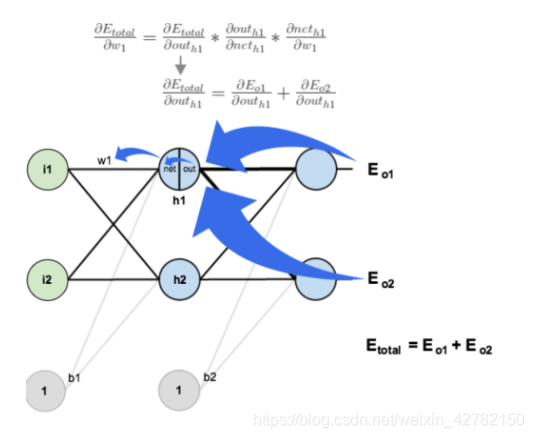
3. 隐藏层----> 输入层的权值更新:
核心原理: 计算隐藏层----> 输入层的权值更新的方法其实和计算输出层----> 隐藏层的权值更新方法类似。区别之处在于,上文在计算总误差对
w
5
w_5
w5的偏导时,是从
o
u
t
o
1
→
n
e
t
o
1
→
w
5
out_{o_1} → net_{o_1}→w_5
outo1→neto1→w5,但在计算隐藏层之间的权值更新时,是从
o
u
t
h
1
→
n
e
t
h
1
→
w
1
out_{h_1} → net_{h_1}→w_1
outh1→neth1→w1,然而
o
u
t
h
1
out_{h_1}
outh1会接受
E
o
1
E_{o_1}
Eo1和
E
o
2
E_{o_2}
Eo2两个地方传递过来的误差,所以此处
E
o
u
t
h
1
E_{out_{h1}}
Eouth1为二者的加和。 求解隐藏层
h
1
h_1
h1到输入层
i
1
i_1
i1的更新权值
w
1
w_1
w1的过程示意图如下:
计算过程:
根据 “链式求导法则”,计算隐藏层 o u t h 1 out_{h_1} outh1对 w 1 w_1 w1的偏导数公式为:
∂ E t o t a l ∂ w 1 = ∂ E t o t a l ∂ o u t h 1 ∗ ∂ o u t h 1 ∂ n e t h 1 ∗ ∂ n e t h 1 ∂ w 1 ↓ ∂ E t o t a l ∂ o u t h 1 = ∂ E o 1 ∂ o u t h 1 + ∂ E o 2 ∂ o u t h 1 \begin{aligned} \frac{\partial E_{total}}{\partial w_1}=&\frac{\partial E_{total}}{\partial{out_{h_1}}}*\frac{\partial{out_{h_1}}}{\partial net_{h_1}}*\frac{{\partial{net_{h_1}}}}{\partial w_1}\\ &\downarrow\\ &\frac{\partial E_{total}}{\partial{out_{h_1}}}=\frac{\partial E_{o_1}}{\partial{out_{h_1}}}+\frac{\partial E_{o_2}}{\partial{out_{h_1}}} \end{aligned} ∂w1∂Etotal=∂outh1∂Etotal∗∂neth1∂outh1∗∂w1∂neth1↓∂outh1∂Etotal=∂outh1∂Eo1+∂outh1∂Eo2
(1)计算 ∂ E t o t a l ∂ o u t h 1 \frac{\partial E_{total}}{\partial{out_{h_1}}} ∂outh1∂Etotal:
接下来,分别计算 ∂ E o 1 ∂ o u t h 1 \frac{\partial E_{o_1}}{\partial{out_{h_1}}} ∂outh1∂Eo1和 ∂ E o 2 ∂ o u t h 1 \frac{\partial E_{o_2}}{\partial{out_{h_1}}} ∂outh1∂Eo2:
根据公式
| —————————————手动分割线————————————— |
∂ E o 1 ∂ o u t h 1 = ∂ E o 1 ∂ o u t o 1 ∗ ∂ o u t o 1 ∂ n e t o 1 ∗ ∂ n e t o 1 ∂ o u t h 1 \begin{aligned} \frac{\partial E_{o_1}}{\partial{out_{h_1}}} &=\frac{\partial E_{o_1}}{\partial{out_{o_1}}}*\frac{\partial{out_{o_1}}}{\partial{net_{o_1}}}*\frac{\partial net_{o_1}}{\partial{out_{h_1}}} \end{aligned} ∂outh1∂Eo1=∂outo1∂Eo1∗∂neto1∂outo1∗∂outh1∂neto1
| —————————————手动分割线————————————— |
其中,
- 第一项
由于
E
o
1
=
1
2
(
t
a
r
g
e
t
o
1
−
o
u
t
o
1
)
2
E_{o_1}=\frac{1}{2}(target_{o_1}-out_{o_1})^2
Eo1=21(targeto1−outo1)2
所以,
∂
E
o
1
∂
o
u
t
o
1
=
−
(
t
a
r
g
e
t
o
1
−
o
u
t
o
1
)
=
−
(
0.01
−
0.75136
)
=
0.74136
\begin{aligned} \frac{\partial E_{o_1}}{\partial out_{o_1}}&=-(target_{o_1}-out_{o_1})\\ &=-(0.01-0.75136)\\ &=0.74136 \end{aligned}
∂outo1∂Eo1=−(targeto1−outo1)=−(0.01−0.75136)=0.74136
- 第二项
由于
o
u
t
o
1
=
1
1
+
e
−
n
e
t
o
1
out_{o_1}=\frac{1}{1+e^{-net_{o_1}}}
outo1=1+e−neto11
所以,
∂
o
u
t
o
1
∂
n
e
t
o
1
=
o
u
t
o
1
(
1
−
o
u
t
o
1
)
=
0.75136
∗
(
1
−
0.75136
)
=
0.1868
\begin{aligned} \frac{\partial out_{o_1}}{\partial net_{o_1}}&=out_{o_1}(1-out_{o_1})\\ &=0.75136*(1-0.75136)\\ &=0.1868 \end{aligned}
∂neto1∂outo1=outo1(1−outo1)=0.75136∗(1−0.75136)=0.1868
- 第三项
由于
n
e
t
o
1
=
w
5
∗
o
u
t
h
1
+
w
6
∗
o
u
t
h
2
+
b
2
∗
1
net_{o_1}=w_5*out_{h_1}+w_6*out_{h_2}+b_2*1
neto1=w5∗outh1+w6∗outh2+b2∗1
因此,
∂
n
e
t
o
1
∂
o
u
t
h
1
=
w
5
=
0.04
\frac{\partial net_{o_1}}{\partial out_{h_1}}=w_5=0.04
∂outh1∂neto1=w5=0.04
- 最后:
∂ E o 1 ∂ o u t h 1 = ∂ E o 1 ∂ o u t o 1 ∗ ∂ n e t o 1 ∂ o u t h 1 = 0.74136 ∗ 0.1868 ∗ 0.40 = 0.055399 \begin{aligned} \frac{\partial E_{o_1}}{\partial{out_{h_1}}} &=\frac{\partial E_{o_1}}{\partial{out_{o_1}}}*\frac{\partial net_{o_1}}{\partial{out_{h_1}}}\\ &=0.74136*0.1868*0.40\\&=0.055399\end{aligned} ∂outh1∂Eo1=∂outo1∂Eo1∗∂outh1∂neto1=0.74136∗0.1868∗0.40=0.055399
同理,可以计算出
∂
E
o
2
∂
o
u
t
h
1
\frac{\partial E_{o_2}}{\partial{out_{h_1}}}
∂outh1∂Eo2:
∂
E
o
1
∂
o
u
t
h
1
=
−
0.019049
\frac{\partial E_{o_1}}{\partial{out_{h_1}}}=-0.019049
∂outh1∂Eo1=−0.019049
最终,二者相加得到总值:
∂
E
t
o
t
a
l
∂
o
u
t
h
1
=
∂
E
o
1
∂
o
u
t
h
1
+
∂
E
o
2
∂
o
u
t
h
1
=
0.055399
+
(
−
0.019049
)
=
0.03635
\begin{aligned} \frac{\partial E_{total}}{\partial{out_{h_1}}}&=\frac{\partial E_{o_1}}{\partial{out_{h_1}}}+\frac{\partial E_{o_2}}{\partial{out_{h_1}}}\\ &=0.055399+(-0.019049)\\ &=0.03635 \end{aligned}
∂outh1∂Etotal=∂outh1∂Eo1+∂outh1∂Eo2=0.055399+(−0.019049)=0.03635
(2)计算 ∂ o u t h 1 ∂ n e t h 1 \frac{\partial{out_{h_1}}}{\partial{net_{h_1}}} ∂neth1∂outh1:
由于
(a)
n
e
t
h
1
=
w
1
∗
i
1
+
w
2
∗
i
2
+
b
1
∗
1
=
0.15
∗
0.05
+
0.2
∗
0.1
+
0.35
∗
1
=
0.3775
\begin{aligned} net_{h_1}&=w_1*i_1+w_2*i_2+b_1*1\\ &=0.15*0.05+0.2*0.1+0.35*1\\ &=0.3775 \end{aligned}
neth1=w1∗i1+w2∗i2+b1∗1=0.15∗0.05+0.2∗0.1+0.35∗1=0.3775
(b)
o
u
t
h
1
=
1
1
+
e
−
n
e
t
h
1
=
0.59327
out_{h_1}=\frac{1}{1+e^{-net_{h_1}}}=0.59327
outh1=1+e−neth11=0.59327
所以,
∂
o
u
t
h
1
∂
n
e
t
h
1
=
o
u
t
h
1
(
1
−
o
u
t
h
1
)
=
0.59327
∗
(
1
−
0.59327
)
=
0.2413
\begin{aligned} \frac{\partial out_{h_1}}{\partial net_{h_1}}&=out_{h_1}(1-out_{h_1})\\ &=0.59327*(1-0.59327)\\ &=0.2413 \end{aligned}
∂neth1∂outh1=outh1(1−outh1)=0.59327∗(1−0.59327)=0.2413
(3)计算
∂
n
e
t
h
1
∂
w
1
\frac{\partial{net_{h_1}}}{\partial w_1}
∂w1∂neth1:
由于
n
e
t
h
1
=
w
1
∗
i
1
+
w
2
∗
i
2
+
b
1
∗
1
\begin{aligned} net_{h_1}&=w_1*i_1+w_2*i_2+b_1*1 \end{aligned}
neth1=w1∗i1+w2∗i2+b1∗1
所以,
∂
n
e
t
h
1
∂
w
1
=
i
1
=
0.05
\begin{aligned} \frac{\partial{net_{h_1}}}{\partial w_1}&=i_1=0.05 \end{aligned}
∂w1∂neth1=i1=0.05
因此,求得 ∂ E t o t a l ∂ w 1 \frac{\partial{E_{total}}}{\partial w_1} ∂w1∂Etotal:
∂ E t o t a l ∂ w 1 = ∂ E t o t a l ∂ o u t h 1 ∗ ∂ o u t h 1 ∂ n e t h 1 ∗ ∂ n e t h 1 ∂ w 1 = 0.03635 ∗ 0.2413 ∗ 0.05 = 0.000438 \begin{aligned} \frac{\partial E_{total}}{\partial w_1}&=\frac{\partial E_{total}}{\partial{out_{h_1}}}*\frac{\partial{out_{h_1}}}{\partial net_{h_1}}*\frac{{\partial{net_{h_1}}}}{\partial w_1}\\ &=0.03635*0.2413*0.05\\ &=0.000438 \end{aligned} ∂w1∂Etotal=∂outh1∂Etotal∗∂neth1∂outh1∗∂w1∂neth1=0.03635∗0.2413∗0.05=0.000438
备注: 为了简化公式,可以使用 δ h 1 δ_{h_1} δh1来表示隐藏层单元 h 1 h_1 h1的误差:
∂ E t o t a l ∂ w 1 = ( ∑ o ∂ E t o t a l ∂ o u t o 1 ∗ ∂ o u t o 1 ∂ n e t o 1 ∗ ∂ n e t o 1 ∂ o u t h 1 ) ∗ ∂ o u t h 1 ∂ n e t h 1 ∗ ∂ n e t h 1 ∂ w 1 = ( ∑ o δ o ∗ w h o ) ∗ o u t h 1 ( 1 − o u t h 1 ) ∗ i 1 = δ h 1 ∗ i 1 \begin{aligned} \frac{\partial E_{total}}{\partial w_1}&=\bigg(\sum_o\frac{\partial E_{total}}{\partial{out_{o_1}}}*\frac{\partial out_{o_1}}{\partial net_{o_1}}*\frac{\partial net_{o_1}}{\partial out_{h_1}}\bigg)*\frac{\partial{out_{h_1}}}{\partial net_{h_1}}*\frac{{\partial{net_{h_1}}}}{\partial w_1}\\ &=\big(\sum_oδ_o*w_{h_o}\big)*out_{h_1}(1-out_{h_1})*i_1\\ &=δ_{h_1}*i_1 \end{aligned} ∂w1∂Etotal=(o∑∂outo1∂Etotal∗∂neto1∂outo1∗∂outh1∂neto1)∗∂neth1∂outh1∗∂w1∂neth1=(o∑δo∗who)∗outh1(1−outh1)∗i1=δh1∗i1
最终, 更新权重 w 1 w_1 w1的计算公式如下:
| —————————————手动分割线————————————— |
w 1 + = w 1 − η ∗ ∂ E t o t a l ∂ w 1 = 0.15 − 0.5 ∗ 0.000438 = 0.14978 \begin{aligned} w_1^+&= w_1-\eta*\frac{\partial E_{total}}{\partial w_1}\\ &=0.15-0.5*0.000438\\ &=0.14978 \end{aligned} w1+=w1−η∗∂w1∂Etotal=0.15−0.5∗0.000438=0.14978
| —————————————手动分割线————————————— |
同理,可以分别求得
w
2
,
w
3
,
w
4
w_2, w_3, w_4
w2,w3,w4的更新权值:
w
2
+
=
0.19956
w
3
+
=
0.24975
w
4
+
=
0.29950
\begin{aligned} w_2^+&= 0.19956\\ w_3^+&= 0.24975\\ w_4^+&= 0.29950 \end{aligned}
w2+w3+w4+=0.19956=0.24975=0.29950


 1200
1200

 被折叠的 条评论
为什么被折叠?
被折叠的 条评论
为什么被折叠?
 到【灌水乐园】发言


