


1.引言
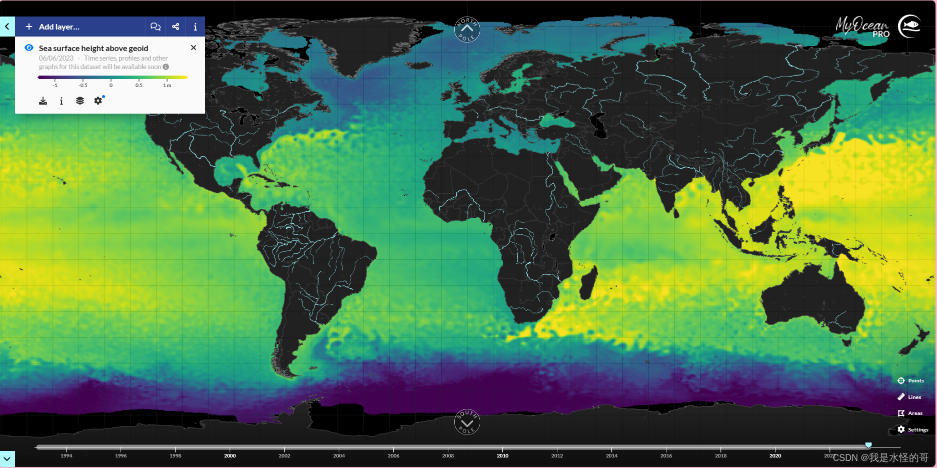
在研究全球海平面变化的问题中,卫星测高获得总的海平面变化,而海平面变化包含质量变化和比容变化。因此测高数据和海洋物理分析数据对于海平面研究至关重要。
测高数据下载网址:
海洋温度和盐度下载网址:
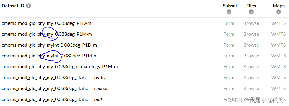
下面介绍的温度和盐度数据的分辨率为0.083°,下载地址:
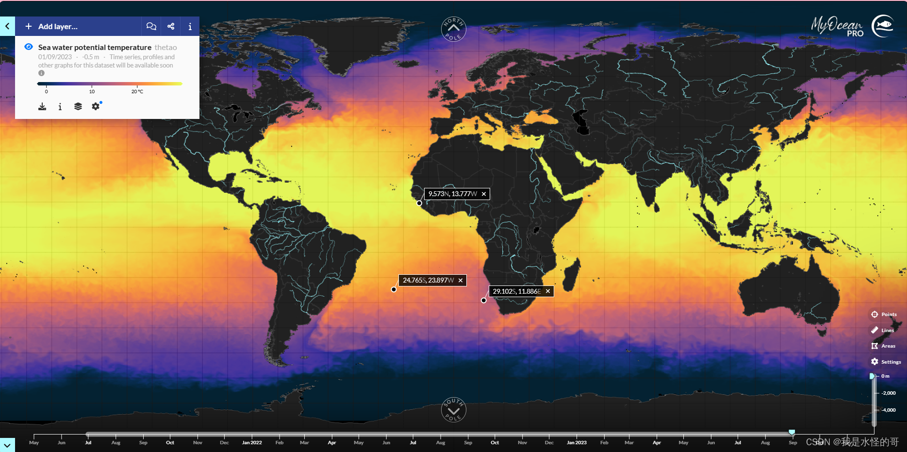
2.数据简介
GLORYS12V1产品是CMEMS全球海洋涡旋解析(水平分辨率1/12°,垂直50个层次)重分析,覆盖高度计数据(从1993年起)。该产品主要基于当前实时全球预报CMEMS系统。模型组件是以NEMO平台为基础,表面由ECMWF ERA-Interim然后是近年来的ERA5重分析驱动。观测数据通过降维卡尔曼滤波器同化。沿轨高度计数据(海平面异常)、卫星海表温度、海冰浓度以及原位温度和盐度垂直剖面被联合同化。此外,3D-VAR方案为温度和盐度的缓慢演变的大尺度偏差提供校正。该产品包括从顶到底的温度、盐度、洋流、海平面、混合层深度和冰参数的日均和月均文件。全球海洋输出文件以标准正则网格显示,水平分辨率为1/12°(约8公里),垂直方向上有50个标准层次。下图展示了数据信息,数据分为每日数据和每月数据,时间跨度为1993年至2023年(最晚访问时间:2024-3-6),其中_my_是1993.1-2021.6,而_myint_是2021.7-至今。
3.数据读取
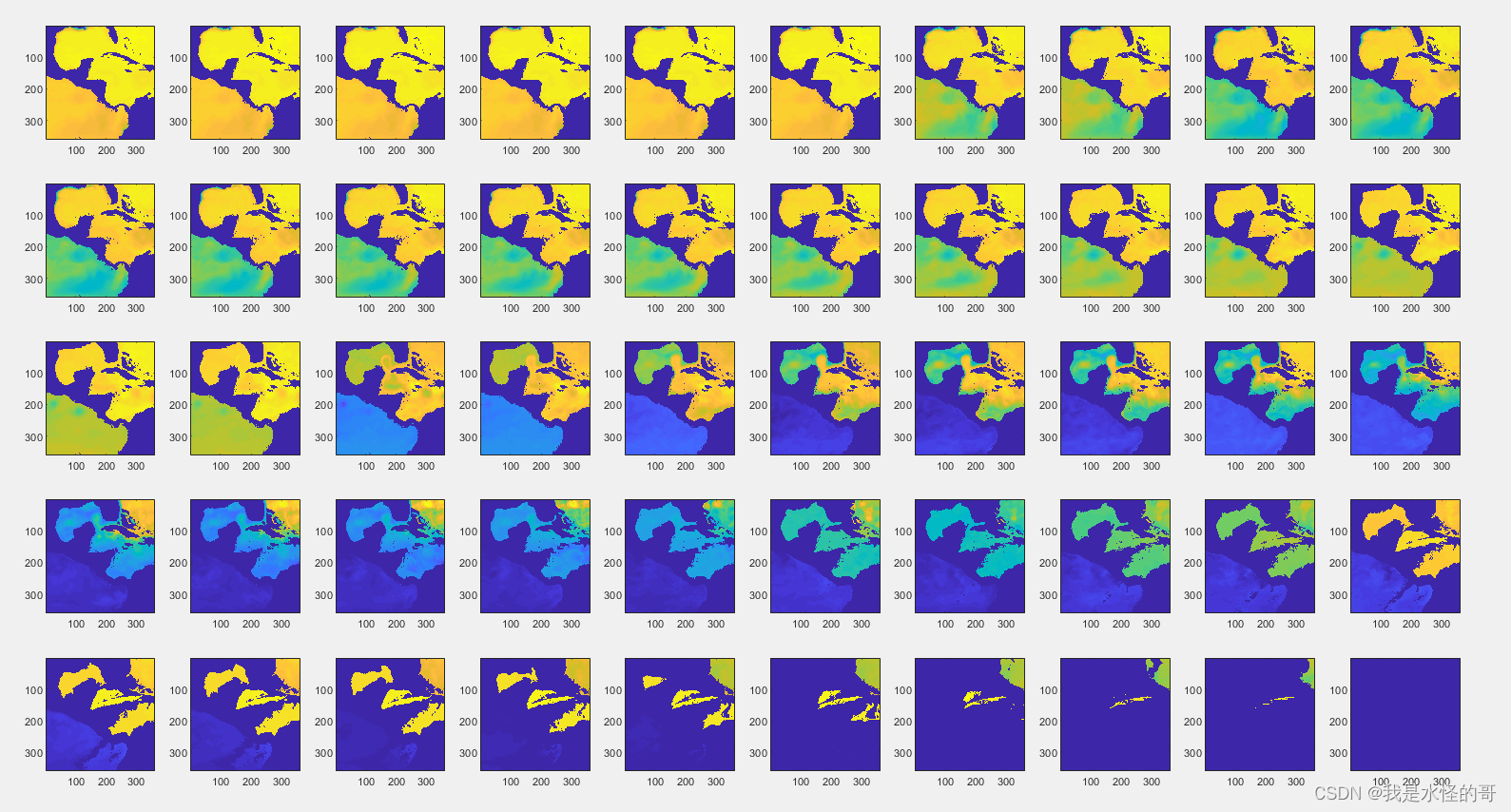
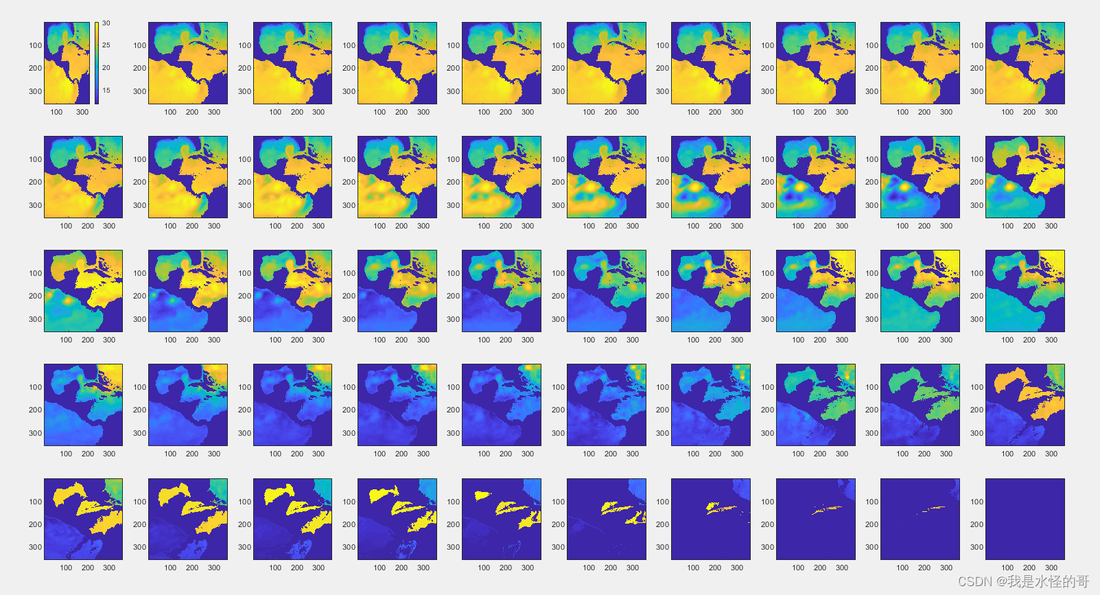
下面以墨西哥湾区域为例,绘制某温度和盐度数据随深度的空间分布:
address_i = 'E:\Ocean_physical\raw\';
GFA = dir(fullfile(address_i,'*nc'));
k = length(GFA);% ncdisp([address,GFA(1).name])
% % load U V velocity
lon = ncread([address_i,GFA(1).name],'longitude');
lat = ncread([address_i,GFA(1).name],'latitude');
[lon,lat] = meshgrid(lon,lat);[m1,n1] = size(lon);
depth = ncread([address_i,GFA(1).name],'depth');A1 = zeros(m1*n1,k+2);
A1(:,1) = reshape(lon,m1*n1,1);
A1(:,2) = reshape(lat,m1*n1,1);
% ind_ = find(A1(:,1)>=110&A1(:,1)<=160&A1(:,2)>=-30&A1(:,2)<=0);
ind_ = find(A1(:,1)>=-100&A1(:,1)<=-70&A1(:,2)>=0&A1(:,2)<=30);
for ii = 1:2
%% read variables
% sea_water_potential_temperature
thetao = ncread([address_i,GFA(ii).name],'thetao');
% sea_water_salinity
so = ncread([address_i,GFA(ii).name],'so');
% eastward_sea_water_velocity
uo = ncread([address_i,GFA(ii).name],'uo');
% northward_sea_water_velocity
vo = ncread([address_i,GFA(ii).name],'vo');
% time
time = ncread([address_i,GFA(ii).name],'time');
dt = datetime(1950,1,1) + hours(time);
[y,m,d] = ymd(dt);
tt(:,1) = time_transfer([y,m,d],1);
%% region mask
for jj = 1:length(depth)
B1 = reshape(thetao(:,:,jj)',m1*n1,1);
aus_region1 = B1(ind_,:);
aus_thetao(:,:,jj) = reshape(aus_region1,361,361);
%%
B2 = reshape(so(:,:,jj)',m1*n1,1);
aus_region2 = B2(ind_,:);
aus_so(:,:,jj) = reshape(aus_region2,361,361);
%%
B3 = reshape(uo(:,:,jj)',m1*n1,1);
aus_region3 = B3(ind_,:);
aus_uo(:,:,jj) = reshape(aus_region3,361,361);
%%
B4 = reshape(vo(:,:,jj)',m1*n1,1);
aus_region4 = B4(ind_,:);
aus_vo(:,:,jj) = reshape(aus_region4,361,361);
end
address_o1 = 'E:\Ocean_physical\output\australia\thetao\';
save([address_o1,'thetao_',num2str(y),'_',num2str(m),'.mat'],'aus_thetao')
address_o2 = 'E:\Ocean_physical\output\australia\so\';
save([address_o2,'thetao_',num2str(y),'_',num2str(m),'.mat'],'aus_so')
address_o3 = 'E:\Ocean_physical\output\australia\uo\';
save([address_o3,'thetao_',num2str(y),'_',num2str(m),'.mat'],'aus_uo')
address_o4 = 'E:\Ocean_physical\output\australia\vo\';
save([address_o4,'thetao_',num2str(y),'_',num2str(m),'.mat'],'aus_vo')
disp(ii)
clear thetao aus_thetao aus_so aus_uo aus_voend
for i = 1:50
subplot(5,10,i)
imagesc(flipud(aus_so(:,:,i)))
endfor i = 1:50
subplot(5,10,i)
imagesc(flipud(aus_thetao(:,:,i)))
end
如果需要计算比容海平面,请参考这篇博文。计算由于海洋温度和盐度变化产生的比容海平面变化-CSDN博客
♥欢迎点赞收藏♥


 1442
1442

 被折叠的 条评论
为什么被折叠?
被折叠的 条评论
为什么被折叠?
 到【灌水乐园】发言


