


说明:
1.写本篇博客的目的之一是方便自己学习记录。
2.本篇博客在前辈的研究基础上稍作修改,代码中有些不明白的地方,需要解释的,请点击下方链接进行学习,本人就不再赘述。
详细介绍用MATLAB实现基于A*算法的路径规划(附完整的代码,代码逐行进行解释)(四)--------固定障碍物,进一步对比-CSDN博客
【路径规划】机器人路径规划之A*算法——四方向_机器人路径规划 a*_A sheep�的博客-CSDN博客
3.本篇博客直接呈现A*算法的matlab代码,如需理解A*算法的原理,推荐下面两篇文章:
在呈现代码前,先简单介绍下本人在前辈给出的程序基础上做出的修改:
①进行A*算法的环境不是n*n的栅格地图,而是n*m的栅格地图 ,这个会影响程序的多处修改。
②进行路径规划的起始点和终止点不是固定的,可以手动输入起始点和终止点的索引值。
③对于非障碍点,有更进一步的定义,在都可经过的情况下,有的方格代价大,有的方格代价小,就好比走山坡代价大,走平坦的路代价小,做路径规划时考虑代价小的进行选择。
A*算法的完整matlab代码:
close all;
clc,clear;    %清除命令窗口的内容

start_index = input("请输入起始点索引值:");
startposind = start_index;

goal_index = input("请输入终止点索引值:");
goalposind = goal_index;

field = [0 1 0 1 0 1 0 1 0 1 0 1 1 1 1 1;
         0 0 0 0 0 0 0 0 0 0 0 1 1 1 1 1;
         2 1 2 1 2 1 2 1 2 1 0 1 1 1 1 1;
         8 1 8 1 8 1 8 1 8 1 0 1 1 1 1 1;
         2 1 2 1 2 1 2 1 2 1 0 1 0 1 0 1;
         0 0 0 0 0 0 0 0 0 0 0 0 0 0 0 0;
         0 1 0 1 0 1 0 1 0 1 0 1 0 1 0 1;];
[n, m] = size(field);

%方格以及障碍物的创建
[field_fli, costchart, fieldpointers] = initializeField(n, m, startposind, goalposind, field);

%路径规划中用到的一些矩阵的初始化
setOpen = startposind;    %用于存放待选点
setOpenCosts = 0;         %存放待选点到起始点的代价
setOpenHeuristics = Inf;  %存放待选点到终点的距离
setClosed = [];           %用于存放下一个进行拓展的父节点
setClosedCosts = [];      %存放拓展的父节点到终点的代价
movementdirections = {'R', 'L', 'D', 'U'};  %进行拓展的移动方向

%生成环境,障碍物,起点,终点
axishandle = createFigure(field_fli, costchart, startposind, goalposind);

%% 本程序的核心,利用循环进行迭代来寻找终止点
while ~max(ismember(setOpen, goalposind)) && ~isempty(setOpen)
    [temp, i] = min(setOpenCosts + setOpenHeuristics);     %temp是拓展出来的最小值,i是最小值在矩阵中的行数

    %把输入的点作为父节点,然后进行拓展找到子节点,并且找到子节点距离起始点和终点的代价
    [costs, heuristics, posinds] = findFValue(setOpen(i), setOpenCosts(i), field_fli, goalposind, 'euclidean');

    setClosed = [setClosed; setOpen(i)];     %将拓展出来的点中代价最小的那个点加到矩阵setClosed中
    setClosedCosts = [setClosedCosts; setOpenCosts(i)];    %将拓展出来的点中代价最小的那个点的代价加到矩阵setClosedCosts中

  %从setOpen中删除刚才放到矩阵setClosed中的那个点
  %如果这个点位于矩阵的内部
  if (i > 1 && i < length(setOpen))
    setOpen = [setOpen(1:i-1); setOpen(i+1:end)];
    setOpenCosts = [setOpenCosts(1:i-1); setOpenCosts(i+1:end)];
    setOpenHeuristics = [setOpenHeuristics(1:i-1); setOpenHeuristics(i+1:end)];

  %如果这个点位于矩阵第一行
  elseif (i == 1)
    setOpen = setOpen(2:end);
    setOpenCosts = setOpenCosts(2:end);
    setOpenHeuristics = setOpenHeuristics(2:end);

  %如果这个点位于矩阵的最后一行
  else
    setOpen = setOpen(1:end-1);
    setOpenCosts = setOpenCosts(1:end-1);
    setOpenHeuristics = setOpenHeuristics(1:end-1);
  end

  %把拓展出来的点中符合要求的点放到setOpen矩阵中,作为待选点
  for j = 1:length(posinds)
    if ~isinf(costs(j))   %该点(方格)不是障碍物

      %判断一下该点是否已经存在于setOpen矩阵或者setClosed矩阵中
      %如果我们要处理的拓展点既不在setOpen矩阵,也不在setClosed矩阵中
      if ~max([setClosed; setOpen] == posinds(j))
        fieldpointers(posinds(j)) = movementdirections(j);
        costchart(posinds(j)) = costs(j);
        setOpen = [setOpen; posinds(j)];
        setOpenCosts = [setOpenCosts; costs(j)];
        setOpenHeuristics = [setOpenHeuristics; heuristics(j)];

      %如果我们要处理的拓展点已经在setOpen矩阵中
      elseif max(setOpen == posinds(j))
        I = find(setOpen == posinds(j));
        %如果通过目前的方法找到的这个点,比之前的方法好(代价小)就更新这个点
        if setOpenCosts(I) > costs(j)
          costchart(setOpen(I)) = costs(j);
          setOpenCosts(I) = costs(j);
          setOpenHeuristics(I) = heuristics(j);
          fieldpointers(setOpen(I)) = movementdirections(j);
        end

      %如果我们要处理的拓展点已经在setClosed矩阵中
      else
        I = find(setClosed == posinds(j));
        %如果通过目前的方法找到的这个点,比之前的方法好(代价小)就更新这个点
        if setClosedCosts(I) > costs(j)
          costchart(setClosed(I)) = costs(j);
          setClosedCosts(I) = costs(j);
          fieldpointers(setClosed(I)) = movementdirections(j);
        end
      end
    end
  end

 if isempty(setOpen)
     break;
 end
  set(axishandle, 'CData', [costchart costchart(:,end); costchart(end,:) costchart(end,end)]);
  set(gca, 'CLim', [0 1.1*max(costchart(costchart < Inf))]);
  drawnow;
end


%调用findWayBack函数进行路径回溯,并绘制出路径曲线
if max(ismember(setOpen, goalposind))
  disp('已找到路径!');
  path = findWayBack(goalposind, fieldpointers);  %进行路径回溯,将回溯结果放于矩阵path中
  plot(path(:,2)+0.5, path(:,1)+0.5, 'Color', 0.2*ones(3,1), 'LineWidth', 4);    %用plot函数绘制路径曲线
  drawnow;
elseif isempty(setOpen)
  disp('未找到路径!');
end

%%
%进行路径回溯,这个函数的输入参数是终止点goalposind和矩阵fieldpointers,输出参数是path
function path = findWayBack(goalposind, fieldpointers)
    [n, m] = size(fieldpointers);
    posind = goalposind;
    [py, px] = ind2sub([n, m], posind);   %将索引值posind转换为坐标值[py,px]
    path = [py px];

    %利用while循环进行回溯,当我们回溯到起始点的时候停止,也就是在矩阵fieldpointers中找到S时停止
    while ~strcmp(fieldpointers{posind},'S')
      switch fieldpointers{posind}

        case 'L' % ’L’ 表示当前的点是由左边的点拓展出来的
          px = px - 1;
        case 'R' % ’R’ 表示当前的点是由右边的点拓展出来的
          px = px + 1;
        case 'U' % ’U’ 表示当前的点是由上面的点拓展出来的
          py = py - 1;
        case 'D' % ’D’ 表示当前的点是由下边的点拓展出来的
          py = py + 1;
      end
      path = [path; py px];
      posind = sub2ind([n m], py, px);  %将坐标值转换为索引值
    end
end


%%
%把输入的点作为父节点,然后进行拓展找到子节点,并且找到子节点距离起始点和终点的代价。
%costs表示拓展的子节点到起始点的代价,heuristics表示拓展出来的点到终止点的代价,posinds表示拓展出来的子节点
function [cost, heuristic, posinds] = findFValue(posind, costsofar, field, goalind, heuristicmethod)
    [n, m] = size(field);
    [currentpos(1), currentpos(2)] = ind2sub([n m], posind);   %将要进行拓展的点(也就是父节点)的索引值拓展成坐标值
    [goalpos(1), goalpos(2)] = ind2sub([n m], goalind);        %将终止点的索引值拓展成坐标值
    %将矩阵cost和heuristic初始化为4x1的无穷大值的矩阵,pos初始化为4x2的值为1的矩阵
    cost = Inf*ones(4,1);
    heuristic = Inf*ones(4,1);
    pos = ones(4,2);

    %拓展方向一
    newx = currentpos(2) - 1; newy = currentpos(1);
    if newx > 0
      pos(1,:) = [newy newx];
      switch lower(heuristicmethod)
        case 'euclidean'
          heuristic(1) = ((goalpos(2) - newx)^2 + (goalpos(1) - newy)^2)^0.5;  %计算终止点距离拓展点的代价或者说是距离
        case 'taxicab'
          heuristic(1) = ((goalpos(2) - newx)^2 + (goalpos(1) - newy)^2)^0.5;
      end
      cost(1) = costsofar + field(newy,newx);   %就是计算出拓展出来的点距离起始点的代价或者说距离
    end

    %拓展方向二
    newx = currentpos(2) + 1; newy = currentpos(1);
    if newx <= m
      pos(2,:) = [newy newx];
      switch lower(heuristicmethod)
        case 'euclidean'
          heuristic(2) = ((goalpos(2) - newx)^2 + (goalpos(1) - newy)^2)^0.5;
        case 'taxicab'
          heuristic(2) = ((goalpos(2) - newx)^2 + (goalpos(1) - newy)^2)^0.5;
      end
      cost(2) = costsofar + field(newy, newx);
    end

    %拓展方向三
    newx = currentpos(2); newy = currentpos(1) - 1;
    if newy > 0
      pos(3,:) = [newy newx];
      switch lower(heuristicmethod)
        case 'euclidean'
          heuristic(3) = ((goalpos(2) - newx)^2 + (goalpos(1) - newy)^2)^0.5;
        case 'taxicab'
          heuristic(3) = ((goalpos(2) - newx)^2 + (goalpos(1) - newy)^2)^0.5;
      end
      cost(3) = costsofar + field(newy, newx);
    end

    %拓展方向四
    newx = currentpos(2); newy = currentpos(1) + 1;
    if newy <= n
      pos(4,:) = [newy newx];
      switch lower(heuristicmethod)
        case 'euclidean'
          heuristic(4) = ((goalpos(2) - newx)^2 + (goalpos(1) - newy)^2)^0.5;
        case 'taxicab'
          heuristic(4) = ((goalpos(2) - newx)^2 + (goalpos(1) - newy)^2)^0.5;
      end
      cost(4) = costsofar + field(newy, newx);
    end
     posinds = sub2ind([n m], pos(:,1), pos(:,2));   %将拓展出来的子节点的坐标值转换为索引值
end


%%
%就是生成环境,障碍物,起始点,终止点等
function [field_fli, costchart, fieldpointers] = initializeField(n, m, startposind, goalposind, field)
   field_fli = flipud(field);   %实现矩阵的上下翻转
   [row, col] = find(field_fli == 1);
   field_fli(sub2ind([n m], row, col)) = Inf;
   [row, col] = find(field_fli == 0);
   field_fli(sub2ind([n m], row, col)) = 1;   %经过方格的代价或者说本身的代价
   [row, col] = find(field_fli == 2);
   field_fli(sub2ind([n m], row, col)) = 2;
   [row, col] = find(field_fli == 8);
   field_fli(sub2ind([n m], row, col)) = 8;
   %生成一个nxm的矩阵costchart,每个元素都设为NaN,就是矩阵初始NaN无效数据
   costchart = NaN*ones(n, m);

   %生成元胞数组
   fieldpointers = cell(n, m);        %生成元胞数组n*m
   fieldpointers{startposind} = 'S';  %将元胞数组的起始点处设为'S'
   fieldpointers{goalposind} = 'G';   %将元胞数组的终止点处设为'G'
   fieldpointers(field_fli == inf) = {0};
end


%%
%环境地图建模
function axishandle = createFigure(field, costchart, startposind, goalposind)
      if isempty(gcbf)
         figure('Position', [450 50 700 700], 'MenuBar','none');
         axes('position', [0.01 0.01 0.99 0.99]);     %本视图窗口建立一个坐标系
      else
         gcf;   %返回当前图像对象的句柄值
         cla;   %从当前坐标区删除包含可见句柄的所有图形对象
      end

      [n, m] = size(field);

      field(field < Inf) = 0;   %将fieid矩阵中没有障碍物的位置处设为0
      pcolor(1:m+1, 1:n+1, [field field(:,end); field(end,:) field(end,end)]);  %多加了一个重复的(由m * n变为 m+1 * n+1 )

      cmap = flipud(colormap('jet'));  %生成的cmap是一个256X3的矩阵,每一行的3个值都为0-1之间数,分别代表颜色组成的rgb值
      cmap(1,:) = zeros(3,1); cmap(end,:) = ones(3,1);   %将矩阵cmap的第一行设为0 ,最后一行设为1
      colormap(flipud(cmap));   %进行颜色的倒转
      hold on;

      axishandle = pcolor(1:m+1, 1:n+1, [costchart costchart(:,end); costchart(end,:) costchart(end,end)]);  %将矩阵costchart进行拓展,插值着色后赋给axishandle

      [goalposy, goalposx] = ind2sub([n, m], goalposind);
      [startposy, startposx] = ind2sub([n, m], startposind);
      plot(goalposx + 0.5, goalposy + 0.5, '-or', 'MarkerSize', 10, 'LineWidth', 10);
      plot(startposx + 0.5, startposy + 0.5, 'p', 'Markersize', 10, 'LineWidth', 5, 'Markerfacecolor', 'r', 'MarkerEdgeColor', 'm');
end
补充说明:
1、对于一开始给出的矩阵field,索引值是从该矩阵左下角开始,即矩阵最左侧一列,从底往上数,索引值是1-7,左侧第二列从底往上是8-14,以此类推。
2、对于方格本身的代价定义如field_fli(sub2ind([n m], row, col)) = 2,可以根据自己的喜好或需求来。
3、对于A*算法,本人还在学习探索中,本篇博客所涉及的代码只是简单的模拟仿真,还需不断改进,不足之处还请见谅,欢迎大家探讨学习。
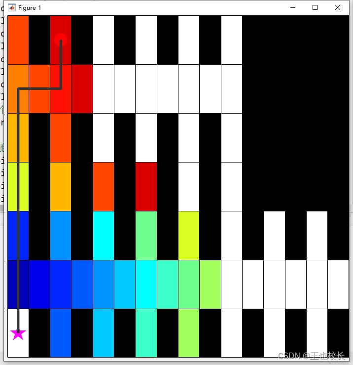
上述代码实现的效果图如下:
起始点索引值为7,终止点索引值为101。 
起始点索引值为1,终止点索引值为21。


 2万+
2万+


 被折叠的 条评论
为什么被折叠?
被折叠的 条评论
为什么被折叠?
 到【灌水乐园】发言


