基于深度卷积神经网络的水果蔬菜图片分类预测

前言

本次主要使用的为深度卷积神经网络，对36种水果蔬菜图片进行模型训练，预测可视化等

首先对数据集进行分析查看，数据集包含2个G的图片，包含3个文件夹，分为训练集、测试集、验证集

其次对数据集图像进行预处理，具体使用为图像增强

接下来使用增强后的数据集对深度卷积神经网络模型进行训练，卷积神经网络对多分类图像处理还是比较强的

最后使用训练的模型使用测试集进行预测评估，随机选取图像可视化结果并展示

1. 导包

import os
import warnings
import numpy as np
import pandas as pd
import seaborn as sns
import matplotlib.pyplot as plt
from tensorflow.keras.preprocessing.image import ImageDataGenerator
from keras.models import Sequential, Model, load_model
from keras.layers import Conv2D, MaxPooling2D, Flatten, Dense
from keras.optimizers import Adam
from keras.preprocessing import image
import matplotlib.pyplot as plt
from keras.layers import concatenate

2. 查看分析数据集

data_dir = '/home/mw/input/fruable7115/frutable/frutable'
train_dir = os.path.join(data_dir, 'train')
test_dir = os.path.join(data_dir, 'test')
validation_dir = os.path.join(data_dir, 'validation')

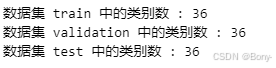
2.1 查看数据集类别数目

def num_of_classes(folder_dir, folder_name) :
    classes = [class_name for class_name in os.listdir(train_dir)]
    print(f'数据集 {folder_name} 中的类别数 : {len(classes)}')

num_of_classes(train_dir, 'train')
num_of_classes(validation_dir, 'validation')
num_of_classes(test_dir, 'test')

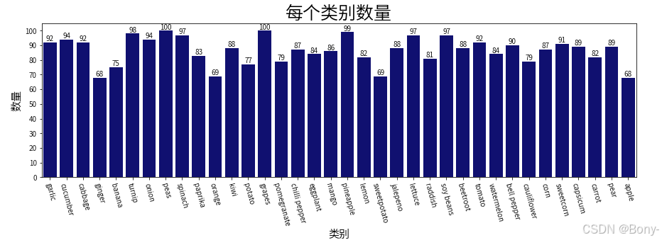
2.2 类别数目

对各个类别进行计数

classes = [class_name for class_name in os.listdir(train_dir)]
count = []
for class_name in classes :
    count.append(len(os.listdir(os.path.join(train_dir, class_name))))

plt.figure(figsize=(15, 4))
ax = sns.barplot(x=classes, y=count, color='navy')
plt.xticks(rotation=285)
for i, value in enumerate(count):
    plt.text(i, value, str(value), ha='center', va='bottom', fontsize=10)
plt.title('每个类别数量', fontsize=25, fontweight='bold')
plt.xlabel('类别', fontsize=15)
plt.ylabel('数量', fontsize=15)
plt.yticks(np.arange(0, 105, 10))
plt.show()

2.3 图像数量

查看各个集的图像总数量

def create_df(folder_path) :
    all_images = []    
    for class_name in classes :
        class_path = os.path.join(folder_path, class_name)
        all_images.extend([(os.path.join(class_path, file_name), class_name) for file_name in os.listdir(class_path)])
    df = pd.DataFrame(all_images, columns=['file_path', 'label'])
    return df

train_df = create_df(train_dir)
validation_df = create_df(validation_dir)
test_df = create_df(test_dir)
print(f'训练集总图像数 : {len(train_df)}')
print(f'验证集总图像数 : {len(validation_df)}')
print(f'测试集总图像数 : {len(test_df)}')

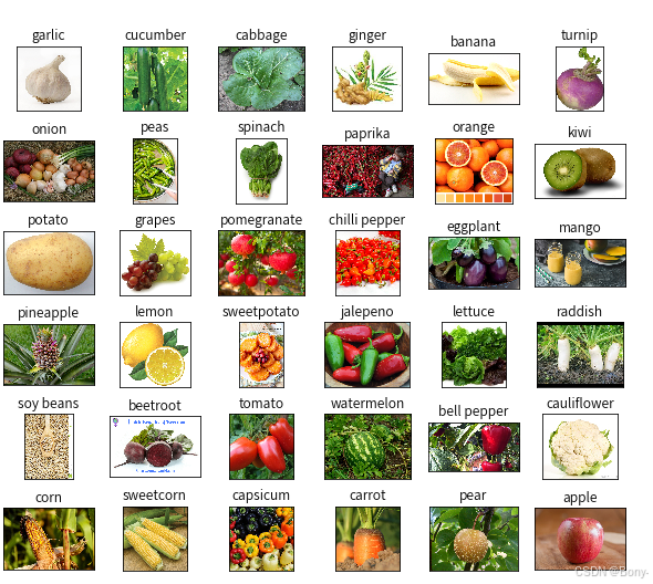
2.4 查看部分图像

df_unique = train_df.copy().drop_duplicates(subset=["label"]).reset_index()

fig, axes = plt.subplots(nrows=6, ncols=6, figsize=(8, 7),
                        subplot_kw={'xticks': [], 'yticks': []})

for i, ax in enumerate(axes.flat):
    ax.imshow(plt.imread(df_unique.file_path[i]))
    ax.set_title(df_unique.label[i], fontsize = 12)
plt.tight_layout(pad=0.5)
plt.show()

3. 图像增强

对数据集进行图像增强，具体意义看下一个cell右边的注释

train_datagen = ImageDataGenerator(
    rescale=1./255,                 # 对图像进行缩放，将像素值标准化到一个较小的范围
    rotation_range=20,              # 随机旋转图像的角度范围，最多旋转 20 度
    width_shift_range=0.2,          # 水平方向上随机移动图像的比例，最多移动图像宽度的 20%
    height_shift_range=0.2,         # 垂直方向同上
    zoom_range=0.1,                 # 随机缩放图像的范围，最多缩放图像 10%
    horizontal_flip=True,           # 随机对图像进行水平翻转
    shear_range=0.1,                # 随机错切变换图像的范围，最多错切图像的 10%
    fill_mode='nearest',            # 对图像进行增强处理时的填充模式，这里设置为最近邻插值
    )
train_generator = train_datagen.flow_from_dataframe(
    dataframe=train_df, 
    x_col='file_path',
    y_col='label',
    target_size=(224, 224),         # 指定将图像调整为的目标大小
    color_mode='rgb',               # 指定图像的颜色模式
    class_mode='categorical',       # 指定分类问题的类型
    batch_size=32, 
    shuffle=True,                 	# 指定是否在每个时期之后打乱数据
    seed=42,
)

validation_datagen = ImageDataGenerator(rescale=1./255,)

validation_generator = validation_datagen.flow_from_dataframe(
    dataframe=validation_df,
    x_col='file_path',
    y_col='label',
    target_size=(224, 224),
    class_mode='categorical',
    batch_size=32,
    seed=42,
    shuffle=False
)

test_datagen = ImageDataGenerator(rescale=1./255,)

test_generator = test_datagen.flow_from_dataframe(
    dataframe=test_df,
    x_col='file_path',
    y_col='label',
    target_size=(224, 224),
    class_mode='categorical',
    batch_size=32,
    seed=42,
    shuffle=False
)

4. 模型训练

选择的是深度卷积神经网络模型，其中输入为（224，224）的RGB图片，输出36个神经元对应36总类别，多分类激活函数选择softmax

# 创建深度卷积神经网络模型
model = Sequential([
    Conv2D(32, (3,3), activation='relu', input_shape=(224, 224, 3)),
    MaxPooling2D((2,2)),
    Conv2D(64, (3,3), activation='relu'),
    MaxPooling2D((2,2)),
    Flatten(),
    Dense(128, activation='relu'),
    Dense(36, activation='softmax') 
])

# 编译模型
model.compile(optimizer=Adam(lr=0.001), loss='binary_crossentropy', metrics=['accuracy'])

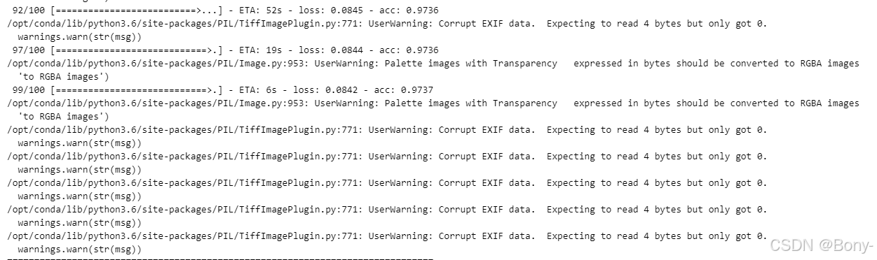
4.1 模型训练

训练过程太长隐藏了，训练也挺久的，可以直接使用我训练好保存的/home/mw/project/fruit.h5

# 训练模型
history = model.fit_generator(
    train_generator,
    steps_per_epoch=100,
    epochs=10,
    validation_data=validation_generator,
    validation_steps=50
)
# 模型保存
model.save('fruit.h5')

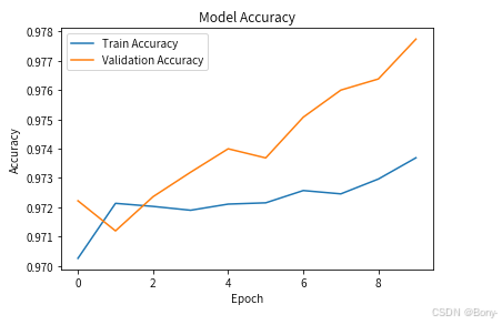
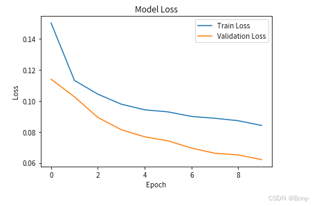
4.2 模型评估

查看模型的准确率和损失值

plt.plot(history.history['acc'], label='Train Accuracy')
plt.plot(history.history['val_acc'], label='Validation Accuracy')
plt.title('Model Accuracy')
plt.ylabel('Accuracy')
plt.xlabel('Epoch')
plt.legend()
plt.show()
# 部分版本使用的是accuracy
# plt.plot(history.history['accuracy'], label='Train Accuracy')
# plt.plot(history.history['val_accuracy'], label='Validation Accuracy')
# plt.title('Model Accuracy')
# plt.ylabel('Accuracy')
# plt.xlabel('Epoch')
# plt.legend()
# plt.show()

plt.plot(history.history['loss'], label='Train Loss')
plt.plot(history.history['val_loss'], label='Validation Loss')
plt.title('Model Loss')
plt.ylabel('Loss')
plt.xlabel('Epoch')
plt.legend()
plt.show()

4.3 使用测试集进行预测评估

可以看出来准确率达到了0.977

# 预测和评估
loss, accuracy = model.evaluate_generator(test_generator, steps=50)
print("Test accuracy:", accuracy)

# 加载模型
model = load_model('fruit.h5')

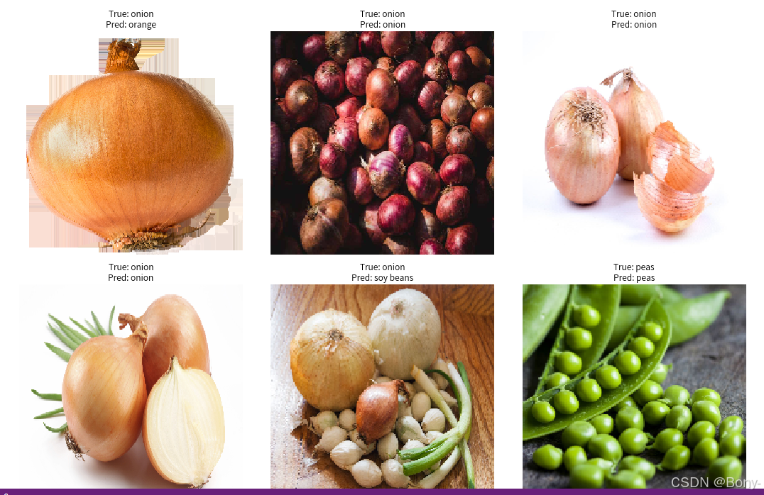
5. 结果展示

随机选择图片进行预测，可视化展示图片、原类别和预测类别
由于每次随机选择的图片不一样，所以多预测几次其实就会发现模型对部分存在明显特征的水果或者蔬菜预测准确率比较好，比如说颜色单一不单一，图片干扰项多不多什么的，感觉很明显

val_images, val_labels = next(validation_generator)

# 进行预测
predictions = model.predict(val_images)
pred_labels = np.argmax(predictions, axis=1)
true_labels = np.argmax(val_labels, axis=1)

# 获取类别映射
class_indices = validation_generator.class_indices
class_names = {v: k for k, v in class_indices.items()}

# 定义显示图像的函数
def display_images(images, true_labels, pred_labels, class_names, num_images=9):
    plt.figure(figsize=(15, 15))
    for i in range(num_images):
        plt.subplot(3, 3, i + 1)
        plt.imshow(images[i])
        true_label = class_names[int(true_labels[i])]
        pred_label = class_names[int(pred_labels[i])]
        plt.title(f"True: {true_label}\nPred: {pred_label}")
        plt.axis('off')
    plt.tight_layout()
    plt.show()

# 调用显示函数
display_images(val_images, true_labels, pred_labels, class_names, num_images=9)

# 若需要完整数据集以及代码请点击以下链接
https://mbd.pub/o/bread/aJaVl55q