Underactuated Robotics lecture 3 笔记 ---Acrobots, cart-poles and quadrotors

3. Introduction

对于低维度的欠驱动系统已经取得了很多的进展，这个部分从低维度开始，逐渐介绍这些主流算法。

3.1 The acrobot

acrobot 机器人，只有elbow关节是有电机的，在shoulder部分是没有电机的，和体操中的单杠类似。
它的典型任务是摆动到最高点并且保持平衡。

3.1.1 Equations of motion

写成标准形式，
$$M(q)\ddot{q}+C(q,\dot{q})\dot{q}={\tau }_g(q)+Bu$$

通过拉格朗日方法计算其中的每一项。

3.2 cart-pole system

典型的小车倒立摆模型如下图。

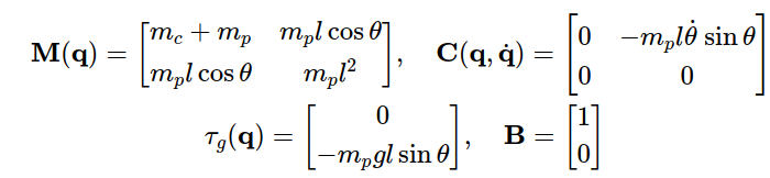
3.2.1 Equations of motion

写成标准形式，对应的项参数如下。

3.3 quadrotors

3.3.1 The planar quadrotor

平面四旋翼的刚体模型如下。
$$\begin{array}{rl}m\ddot{x}& =-(u_1+u_2)sin\theta \\ m\ddot{y}& =(u_1+u_2)cos\theta -mg\\ I\ddot{\theta }& =r(u_1-u_2)\end{array}$$

3.4 Balancing

控制acrobot 和 cart-pole系统，在unstable fixed point附件，设计线性控制器平衡系统，步骤：
1）在固定点附近线性化；
2）评估线性系统的能控性；
3）使用LQR设计线性控制器；

3.4.1 对动力学方程进行线性化

在fixed point附近进行泰勒展开，
$$\dot{x}=f(x,u)\approx f(x^{\ast },u^{\ast })+\frac{\partial f}{\partial x}{|}_{x=x^{\ast },u=u^{\ast }}(x-x^{\ast })+\frac{\partial f(x,u)}{\partial u}{|}_{x=x^{\ast },u=u^{\ast }}(u-u^{\ast })$$

接下来将动力学方程转换成状态转移方程，设x=$[q;\dot{q}]$,
$$\begin{array}{rl}\dot{x}& =\left[\begin{array}{c}\dot{q}\\ M^{-1}(q)[{\tau }_g(q)+B(q)u-C(q,\dot{q})\dot{q}]\end{array}\right]\\ & \approx A_{lin}(x-x^{\ast })+B_{lin}(u-u^{\ast })\end{array}$$

对矩阵中的项关于$(q,\dot{q},u)$展开，并且利用fixed point的一些特殊性质如：
$$\begin{array}{rlr}{\ddot{q}}^{\ast }& ={\tau }_g(q^{\ast })+B(q^{\ast })u-C(q^{\ast },{\dot{q}}^{\ast })\dot{q^{\ast }}& =0\\ {\dot{q}}^{\ast }& =0& \\ C(q^{\ast },{\dot{q}}^{\ast })& =0& \end{array}$$

得到

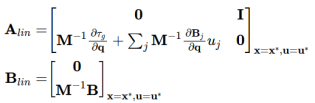
对于很多系统，B是constant 矩阵，对应的线性化之后的矩阵更加简单了。

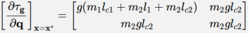
• Linearation of the acrobot
  
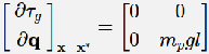
• Linearization of the cart-pole system
  
  得到线性化结果之后，可以通过矩阵的特征值判断稳定性，或者其他传统控制的办法。
• 为什么搞线性化？
  1）在第2节内容，如果是一个全驱动的系统，完全可以通过模型转换的方法。把非线性系统变换成一个线性系统。
  2）对于欠驱动系统，线性化以后，可以用一些经典控制理论，LQR和PID。

3.4.2 Controllability of linear system

能控性，考察系统是否可以到达状态空间中的任意状态，先看能控的定义。

课程提供了一种直觉理解的方法，通过引入特征向量将问题变得更清晰。

• non-repeated eigenvalues
  状态矩阵A的特征向量为$v_i$,特征值为${\lambda }_i$
  $$\begin{array}{rl}A{v}_i& ={\lambda }_i{v}_i\\ AV& =V\Lambda \end{array}$$
  将状态空间中的状态量映射到特征向量组成的空间中：
  $$\begin{array}{rl}x& =Vr\\ \dot{r}& =V^{-1}\dot{x}\\ & =V^{-1}(Ax+Bu)\\ & =V^{-1}AVr+V^{-1}Bu\\ & =\Lambda r+V^{-1}Bu\\ {\dot{r}}_i& ={\lambda }_i{r}_i+\sum _j{\beta }_{ij}{u}_j\end{array}$$
  只要保证$V_i,\exists {\beta }_{ij}\ne 0$,能满足能控性。
• general solution
  general solution就是传统控制理论上的能控的定义，省略不表。
• controllability vs underactuated
  对于典型的欠驱动系统，acrobot 和cartpole 系统，在unstable fixed point附近却是能控的。这说明了我们用一个LQR这样的控制器就能搞定他们了。
• $现有的进展和问题$
  

3.5 partial feedback linearization

借用全驱动的直接线性化的方法，探索一下如果进行局部线性化会这么样。根据控制器是否线性化驱动关节，分为：
collocated partial feedback linearization 和non-collocated partial feedback linearization。

3.5.1 PFL for the cart-pole system

先建立一个简化的cart-pole 动力学方程
$$\begin{array}{rl}2\ddot{x}+\ddot{\theta }cos\theta -{\dot{\theta }}^{2}sin\theta & =f_x\\ \ddot{x}cos\theta +\ddot{\theta }+sin\theta & =0\end{array}$$

• collocated
  把第一项中，欠驱动关节的加速度$\ddot{\theta }$替换掉，得到下面的形式
  $$\begin{array}{rl}\ddot{\theta }& =-\ddot{x}c-s\\ \ddot{x}(2-c^2)& -sc-{\dot{\theta }}^{2}s=f_x\end{array}$$
  通过控制$f_x$可以得到目标加速度${\ddot{x}}^d$，得到下面的形式：
  $$\begin{array}{rl}\ddot{x}& ={\ddot{x}}^d\\ \ddot{\theta }& =-{\ddot{x}}^{d}c-s\end{array}$$
  现在这个模型可以看成是单倒立摆，受到输入力矩$-{\ddot{x}}^{d}c$。
• non-collocated
  将第一项中的，驱动关节的加速度$\ddot{x}$替换掉，得到下面的形式
  $$\begin{array}{rl}\ddot{x}& =-\frac{\ddot{\theta }+s}{c}\\ \ddot{\theta }(c-\frac{2}{c})& -2tan\theta -{\dot{\theta }}^{2}s=f_x\end{array}$$
  同样的，此时控制f_x可以得到目标$\ddot{\theta }$,有
  $$\begin{array}{rl}\ddot{\theta }& ={\ddot{\theta }}^d\\ \ddot{x}& =-\frac{{\ddot{\theta }}^d+s}{c}\end{array}$$
  需要注意的是，要检查$cos\theta \ne 0$

3.5.2 General form

针对欠驱动系统动力学方程的特殊性，令$M(q)=\left[\begin{array}{cc}{M}_{11}& M_{12}\\ M_{21}& M_{22}\end{array}\right]$, $\tau ={\tau }_g-C\dot{q}$,将基本动力学公式转换成下面的形式。$q_1$代表passive joints, $q_2$代表actuated joints,并且M是正定矩阵。
$$\begin{array}{rl}{M}_{11}{\ddot{q}}_1+M_{12}{\ddot{q}}_2& ={\tau }_1\\ M_{21}{\ddot{q}}_1+M_{22}{\ddot{q}}_2& ={\tau }_2+u\end{array}$$

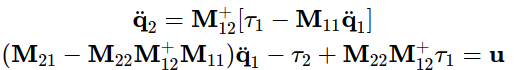
• Collocated linearization
  $$\begin{array}{rl}{\ddot{q}}_1& =M_{11}^{-1}({\tau }_1-M_{12}{\ddot{q}}_2)\\ (M_{22}-M_{21}{M}_{11}^{-1}{M}_{12}){\ddot{q}}_2& -{\tau }_2+M_{21}{M}_{11}^{-1}{\tau }_1=u\end{array}$$
• Non-collocated linearization
  
• task-space partial feedback linearization
  考虑如何控制末端轨迹，
  $$\begin{array}{rl}y& =h(q)\\ \dot{y}& =H\dot{q}=\left[\begin{array}{cc}\frac{\partial h}{\partial q_1}& \frac{\partial h}{\partial q_2}\end{array}\right]\dot{q}\\ \ddot{y}& =\dot{H}\dot{q}+H_1{\ddot{q}}_1+H_2{\ddot{q}}_2\\ & =\dot{H}\dot{q}+H_1(M_{11}^{-1}[{\tau }_1-M_{12}{\ddot{q}}_2])+H_2{\ddot{q}}_2\end{array}$$
  最终得到下面的公式：
  
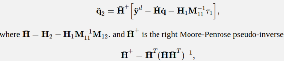
  这里非常关键的是，$\bar{H}$的秩，如果驱动关节的自由度大于末端的自由度，能保证$\bar{H}$的列数大于行数。
  部署顺序：
  1）规划末端的轨迹；
  2）添加反馈控制器；
  $${\ddot{y}}^d={\ddot{y}}_r^d+K_d({\dot{y}}^d-\dot{y})+K_p(y^d-y)$$
  3）反算驱动关节的加速度；
  4）在利用collocated linearization 反算系统的输入量；
• examples
  1)cart-pole system
  只控制cart-pole的竖直高度，轨迹规划：
  $$\begin{array}{rl}y& =h(q)=-lcos(\theta )\\ \dot{y}& =l\dot{\theta }sin\theta \\ y^d(t)& =0.5l+0.25lsin(t)\end{array}$$
  2 ) task-space partial linearization 提供了一个框架，非常方便的得到collocated 和non-collocated 结果。
  $$\begin{array}{rl}y& =q_2\\ H_1=0,H_2=I,& \dot{H}=0,\bar{H}=I,{\bar{H}}^{+}=I\\ \ddot{q_2}& ={\ddot{q}}_2^d\end{array}$$
  带入执行关节加速度和输入u关系公式，即可得到collocation的结果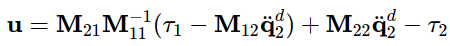
  同理，得到non-collocation的形式，但是需要注意为例满足存在唯一解的条件，要求$rank(M_{12})=l(numofpassivedegress)$

3.6 swing-up control

这一章的最后提供了一套最基本的框架，来解决两个典型的欠驱动问题。欠驱动问题的难点在于很难把系统搞到上一章提高的phase portait上的一个稳定的轨道上，然后再用LQR处理。
这里的系统比较简单，用energy shaping就完成了phase portait上换轨的任务，这才是关键。

3.6.2 Cart-pole

先简化模型，
$$\begin{array}{rl}\ddot{x}& ={\ddot{x}}^d\\ \ddot{\theta }& =-{\ddot{x}}^{d}c-s\end{array}$$
带入energy-shaping 的公式
$$\begin{array}{rl}E(x)& =\frac{1}{2}{\dot{\theta }}^2-cos\theta \\ E^d& =1,\tilde{E}(x)=E(x)-E^d\\ \dot{\tilde{E}}(x)& =\dot{E}(x)=\dot{\theta }\ddot{\theta }+\dot{\theta }s\\ & =\dot{\theta }(-{\ddot{x}}^{d}c-s)+\dot{\theta }s\\ & =-\dot{\theta }{\ddot{x}}^{d}c\end{array}$$
令${\ddot{x}}^d=k\dot{\theta }cos\theta \tilde{E}$, k>0,有
$$\dot{\tilde{E}}=-k{\dot{\theta }}^{2}co{s}^2\theta \tilde{E}$$

理论可以证明$\tilde{E}\to 0$
设计PD控制器，${\ddot{x}}^d=k\dot{\theta }cos\theta \tilde{E}-k_{p}x-k_d\dot{x}$
本来根据collocation的公式，有$a{\ddot{x}}^d+b=u$,因为这里有需要认为调节的增益项$k,k_p,k_d$，所以可以直接令${\ddot{x}}^d=u$。

总结一下，第二章的时候我们解决不了这个问题，只能保证倒立摆的能量完成换轨，因为没有小车的线性模型，没法同时控制小车，现在有了partial feedback linearization。完成了小车控制和倒立摆能量换轨。
energy-shaping 控制方法灵活性太高，并且它还没有考虑到输入受限和状态受限这种约束。