基于标准粒子群优化算法的TSP搜索算法

一、理论基础

在TSP问题中，粒子的位置可以使用路径来表示，速度如何表示却是一个难题。基本粒子群算法的速度和位置更新公式不再适用，因此本文重新定义了速度和位置的更新公式。
基本粒子群算法速度位置更新公式：$$V_{id}^{k+1}=\omega V_{id}^k+c_1{r}_1(P_{id}^k-X_{id}^k)+c_2{r}_2(P_{gd}^k-X_{id}^k)\text{\hspace{1em}(1)}$$$$X_{id}^{k+1}=X_{id}^k+V_{k+1_{id}}\text{\hspace{1em}(2)}$$
本文重新定义了速度，以及三个运算规则：位置-位置，常数×速度，位置+速度

速度

速度定义为交换序列，$position1+velocity=position2$意思是$position1$通过$velocity$(速度)这个交换序列变成$position2$，速度中每一个索引对应的数字表示为$position1$中索引为该数字的城市与$position1$中索引为速度索引的城市对调，例如：$$position1=[54321]，position2=[12345]$$由于$$position2(1)=position1(5)$$因此$position1(1)$与$position1(5)$互换位置，$velocity(1)=5$
交换位置之后：$$position1=[14325]，position2=[12345]$$又因为$$position2(2)=position1(4)$$因此$position1(2)$与$position1(4)$互换位置，$velocity(2)=4$
交换位置之后：$$position1=[12345]，position2=[12345]$$又因为$$position2(3)=position1(3)$$因此$position1(3)$与$position1(3)$互换位置(相当于没做)，$velocity(3)=3$
由此可以推导，$velocity=[54345]$
定义$position2-position1$即为速度。

常数×位置

定义为：速度中的每一个值以该常数的概率保留，避免过早陷入局部最优解。

二、MATLAB程序实现

1、问题描述

TSP(traveling salesman problem,旅行商问题)是典型的NP完全问题，即其最坏情况下的时间复杂度随着问题规模的增大按指数方式增长，到目前为止还未找到一个多项式时间的有效算法。
TSP问题可描述为：已知$n$个城市相互之间的距离，某一旅行商从某个城市出发访问每个城市有且仅有一次，最后回到出发城市，如何安排才使其所走路线距离最短。简言之，就是寻找一条最短的遍历$n$个城市的路径，或者说搜索自然子集 X = { 1 , 2 , ⋯   , n } X=\{1,2,\dotsm,n\} X={1,2,⋯,n}($X$的元素表示对$n$个城市的编号)的一个排列 π ( X ) = { V 1 , V 2 , ⋯   , V n } π(X)=\{V_1,V_2,\dotsm,V_n\} π(X)={V1​,V2​,⋯,Vn​}，使得$$T_d=\sum _{i=1}^{n+1}d(V_i,V_{i+1})+d(V_n,V_1)$$取得最小值，其中$d(V_i,V_{i+1})$表示城市$V_i$到城市$V_{i+1}$的距离。

2、代码实现

• 计算粒子适应度函数

function fitness = fun(pop, citys, D)
%% 计算粒子适应度函数
% 输入：pop      粒子群位置     citys   城市坐标   D    距离矩阵
% 输出：fitness  粒子的适应度值
m = size(pop, 1);
n = size(citys, 1);
fitness = zeros(m, 1);
for i = 1:m
    for j = 1:n-1
        fitness(i) = fitness(i) + D(pop(i, j), pop(i, j+1));
    end
    fitness(i) = fitness(i) + D(pop(i, end), pop(i, 1));
end

• 记录将pop变成best的交换序列的函数

function change = position_minus_position(best, pop)
%% 记录将pop变成best的交换序列
for i = 1:size(best, 1)
    for j = 1:size(best, 2)
        change(i, j) = find(pop(i, :)==best(i, j));   % 找到最佳值索引
        temp = pop(i, j);
        pop(i, j) = pop(i, change(i, j));
        pop(i, change(i, j)) = temp;                  % 交换
    end
end

• 利用速度记录的交换序列进行位置修正的函数

function pop = position_plus_velocity(pop, V)
%% 利用速度记录的交换序列进行位置修正
for i = 1:size(pop,1)
    for j = 1:size(pop,2)
        if V(i, j) ~= 0
            temp = pop(i, j);
            pop(i, j) = pop(i, V(i,j));
            pop(i, V(i,j)) = temp;
        end
    end
end

• 以一定概率保留交换序列的函数

function change = constant_times_velocity(constant, change)
%% 以一定概率保留交换序列
for i = 1:size(change, 1)
    for j = 1:size(change, 2)
        if rand > constant
            change(i, j) = 0;
        end
    end
end

• 主函数

%% 1.清空环境变量
clear;
clc;

%% 2.导入数据
load citys_data.mat;     % 数据集的变量名为citys

%% 3.计算城市间相互距离
n = size(citys, 1);
D = Distance(citys);

%% 4.初始化参数
c1 = 0.1;                           % 个体学习因子
c2 = 0.075;                         % 社会学习因子
w = 1;                              % 惯性权重
m = 500;                            % 粒子数量
pop = zeros(m, n);                  % 粒子位置
V = zeros(m,n);                     % 粒子速度
gen = 1;                            % 迭代计数器
maxgen = 2000;                      % 迭代次数
fitness = zeros(m, 1);              % 适应度函数值
pbest = zeros(m, n);                % 个体极值路径
fitnesspbest = zeros(m,1);          % 个体极值
gbest = zeros(maxgen, n);           % 群体极值路径
fitnessgbest = zeros(maxgen, 1);    % 群体极值
Length_ave = zeros(maxgen, 1);      % 各代路径的平均长度
ws = 0.9;                           % 惯性权重最大值
we = 0.4;                           % 惯性权重最小值

%% 5.产生初始粒子
% 随机产生粒子初始位置和速度
for i = 1:m
    pop(i, :) = randperm(n);
    V(i, :) = randperm(n);
end
% 计算粒子适应度函数值
fitness = fun(pop, citys, D);
% 计算个体极值和群体极值
fitnesspbest = fitness;         % 个体极值适应度值
pbest = pop;                    % 个体极值
[fitnessgbest(1), min_index] = min(fitness);
gbest(1, :) = pop(min_index, :);
Length_ave(1) = mean(fitness);

%% 6.迭代寻优
while gen < maxgen
    gen
    %% 更新迭代次数与惯性权重
    gen = gen+1;
    w = ws - (ws-we)*(gen/maxgen)^2;   

    %% 更新速度
    % 个体极值更新部分
    change1 = position_minus_position(pbest, pop);
    change1 = constant_times_velocity(c1, change1);
    % 群体极值修正部分
    change2 = position_minus_position(repmat(gbest(gen-1, :), m, 1), pop);
    change2 = constant_times_velocity(c2, change2);
    % 原速度部分
    V = constant_times_velocity(w, V);
    % 修正速度
    for i = 1:m
        for j = 1:n
            if change1(i, j) ~= 0
                V(i, j) = change1(i, j);
            end
            if change2(i, j) ~= 0
                V(i, j) = change2(i, j);
            end
        end
    end

    %% 更新位置
    pop = position_plus_velocity(pop, V);

    %% 适应度函数值更新
    fitness = fun(pop, citys, D);
    %% 个体极值与群体极值更新
    % 个体极值更新
    for i = 1:m
        if fitness(i) < fitnesspbest(i)
            fitnesspbest(i) = fitness(i);
            pbest(i, :) = pop(i, :);
        end
    end
    % 群体极值更新
    [minvalue, min_index] = min(fitness);
    if minvalue < fitnessgbest(gen-1)
        fitnessgbest(gen) = minvalue;
        gbest(gen, :) = pop(min_index, :);
    else
        fitnessgbest(gen) = fitnessgbest(gen-1);
        gbest(gen, :) = gbest(gen-1, :);
    end
    % 记录每代的平均路径长度
    Length_ave(gen)=mean(fitness);
end

%% 7.结果显示
[Shortest_Length, index] = min(fitnessgbest);
Shortest_Route = gbest(index, :);
disp(['最短距离:' num2str(Shortest_Length)]);
disp(['最短路径:' num2str([Shortest_Route Shortest_Route(1)])]);

%% 8.绘图
figure(1)
plot([citys(Shortest_Route, 1); citys(Shortest_Route(1), 1)],...
     [citys(Shortest_Route, 2);citys(Shortest_Route(1), 2)], 'o-', 'linewidth', 2);
grid on
for i = 1:size(citys,1)
    text(citys(i, 1), citys(i, 2), ['   ' num2str(i)]);
end
text(citys(Shortest_Route(1), 1), citys(Shortest_Route(1), 2),'       起点');
text(citys(Shortest_Route(end),1), citys(Shortest_Route(end), 2),'       终点');
xlabel('城市位置横坐标')
ylabel('城市位置纵坐标')
title(['粒子群算法优化路径(最短距离:' num2str(Shortest_Length) ')'])
figure(2)
plot(1:maxgen, fitnessgbest, 'b', 1:maxgen, Length_ave, 'r:', 'linewidth', 2);
legend('最短距离', '平均距离')
xlabel('迭代次数')
ylabel('路径距离')
title('各代最短距离与平均距离对比')

• 结果显示
  Command Window中显示的结果为：

最短距离:17515.8526
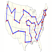
最短路径:1  15  14  12  30  29  11  13   7   2   4  19  17  18   3  10   9   8  16   5   6  23  24  25  20  21  22  26  28  27  31   1

• 绘图
  粒子群算法优化路径变化如图1所示。
  

图1 PSO算法优化路径 各代最短距离与平均距离对比如图2所示。

图2 各代最短距离与平均距离对比

代码下载链接：https://download.csdn.net/download/weixin_43821559/85224716

三、参考文献

[1] Leung_ZY. 遗传算法、蚁群算法、粒子群算法解决TSP总结 matlab代码. CSDN博客.
[2] 心升明月. 基于粒子群优化算法的函数寻优算法. CSDN博客.
[3] Xia T, Guo W, Chen G. An Improved Particle Swarm Optimization for Data Streams Scheduling on Heterogeneous Cluster[C]. International Conference on Advances in Computation & Intelligence. Springer Berlin Heidelberg, 2007: 393-400.