【机器学习】（六）线性模型：线性回归、岭回归、Lasso；Logistic回归、线性SVM

回归问题

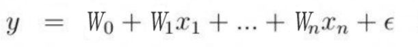
线性模型利用输入特征的线性函数（一次函数）进行预测。
线性函数有两个参数：w[n]斜率（每个特征的系数），y轴偏移量。输出是预测结果。
Θ是权重组成的向量。

可视化：mglearn.plots.plot_linear_regression_wave()

对单一特征预测结果是一条直线。2个特征是一个平面，更高维度（更多特征）时是一个超平面。

解析解方法求解线性回归

# 代码实战解析解求解模型的方法
# numpy是去做数值计算的
import numpy as np
# matplotlib是关于绘图的
import matplotlib.pyplot as plt

np.random.seed(42)

# 回归，有监督的机器学习，X，y
# rand 是随机均匀分布，100行1列
X1 = 2*np.random.rand(100, 1)
X2 = 3*np.random.rand(100, 1)
# 这里要模拟出来的数据y是代表真实的数据，所以也就是y_hat+error,100行1列
# np.random.randn(100, 1)是设置 error，randn 是标准正太分布，符合误差服从均值为 0 的正太分布
y = 5 + 4*X1 + 3*X2 + np.random.randn(100, 1)

# 多元线性回归中，W 的个数其实是和 X 特征的数量
# 为了去求解W0截距项，我们给X矩阵一开始加上一列全为1的X0，100行3列
# np.c_是按行连接两个矩阵，就是把两矩阵左右相加，要求行数相等。
X_b = np.c_[np.ones((100, 1)), X1, X2]

# 实现解析解的公式来求解θ
# .T 就是 transpose 转置的作用，dot 就是向量点乘， np.linalg.inv 是矩阵求逆
θ = np.linalg.inv(X_b.T.dot(X_b)).dot(X_b.T).dot(y)
print(θ)

# 使用模型去做预测
X_new = np.array([[0, 0],
                  [2, 3]])
X_new_b = np.c_[np.ones((2, 1)), X_new]
print(X_new_b)
y_predict = X_new_b.dot(θ)
print(y_predict)

# 绘图进行展示真实的数据点和我们预测用的模型
plt.plot(X_new[:, 0], y_predict, 'r-')
plt.plot(X1, y, 'b.')
plt.axis([0, 2, 0, 25])
plt.show()

# 三维图
from mpl_toolkits.mplot3d import Axes3D
fig = plt.figure()
ax = Axes3D(fig)
ax.plot_trisurf(X1.reshape(100), X2.reshape(100), y.reshape(100))
plt.show()

线性回归OLS：LinearRegression

线性回归/普通最小二乘法/OLS，寻找参数w、b是的训练集预测值与真实的回归目标值y之间的均方差误差（差的平方和除以样本数）最小。
没有参数，无法控制模型复杂度。

在wave数据集的应用

from sklearn.linear_model import LinearRegression
from sklearn.model_selection import train_test_split

x, y = mglearn.datasets.make_wave(n_samples=60)
x_train, x_test, y_train, y_test = train_test_split(x, y, random_state=42)

lr = LinearRegression().fit(x_train, y_train)

print(lr.coef_) # 保存权重参数。[0.39390555]
print(lr.intercept_) # 保存截距参数。-0.031804343026759746

print(lr.score(x_train, y_train)) # 0.6700890315075756
print(lr.score(x_test, y_test)) # 0.65933685968637

scikit-learn将训练中取出的值保存在以下划线结尾的属性中。
coef_属性：保存斜率参数。NumPy数组。
intercept_属性：保存偏移/截距参数。浮点数。

训练集和测试集分数都较低，可能存在欠拟合，因为一维数据模型简单。

在boston数据集的应用

x, y = mglearn.datasets.load_extended_boston()
x_train, x_test, y_train, y_test = train_test_split(x, y, random_state=0)
lr = LinearRegression().fit(x_train, y_train)

print(lr.score(x_train, y_train)) # 0.952051960903273
print(lr.score(x_test, y_test)) # 0.6074721959665708

训练集预测准确，测试集预测比较不准确。存在过拟合，因为模型过于复杂（103特征）。

因此应该找一个可以控制复杂度的模型↓

岭回归：Ridge

岭回归的预测公式和OLS相同，在系数w的选择要拟合附加约束【正则化】。
正则化是指对模型做显示约束，以避免过度拟合。
岭回归使用L2正则化：系数尽量小，即w所有元素都应接近于0。

在boston数据集的应用

from sklearn.linear_model import Ridge

# alpha=1.0
ridge = Ridge().fit(x_train, y_train)
print(ridge.score(x_train, y_train)) # 0.885796658517094
print(ridge.score(x_test, y_test)) # 0.7527683481744755

# alpha=0.1
ridge01 = Ridge(alpha=0.1).fit(x_train, y_train)
print(ridge01.score(x_train, y_train)) # 9282273685001985
print(ridge01.score(x_test, y_test)) # 0.772206793647982

# alpha=10
ridge10 = Ridge(alpha=10).fit(x_train, y_train)
print(ridge10.score(x_train, y_train)) # 7882787115369614
print(ridge10.score(x_test, y_test)) # 0.635941148917731

比起线性回归0.95-0.6，岭回归0.88-0.75，更加不容易过拟合，泛化性能更好。

Ridge模型通过alpha参数权衡简单性（系数接近于0）与训练集新能之间做出权衡。默认alpha=1.0。
增大alpha会提高泛化性能，降低训练集性能。
alpha特别小时，系数不受到约束，Ridge≈LinearRegression。
大alpha对应的coef_元素（保存斜率参数的NumPy数组）比小alpha对应的元素参数小。

固定alpha的值，增大数据量，也可以达到防止过拟合（数据量大难以记住所有数据），正则化将不再重要。
可视化：mglearn.plots.plot_ridge_n_samples()

lasso

lasso和Ridge一样也是正则化线性回归，约束系数使其接近于0。
使用L1正则化：某些系数=0（对应特征被模型完全忽略）

在boston数据集的应用

from sklearn.linear_model import Lasso

# alpha = 1.0
lasso = Lasso().fit(x_train, y_train)
print(lasso.score(x_train, y_train)) # 0.29323768991114607
print(lasso.score(x_test, y_test)) # 0.20937503255272294
print(np.sum(lasso.coef_!=0)) # 系数不为0的w。4

# alpha = 0.01
lasso001 = Lasso(alpha=0.01, max_iter=100000).fit(x_train, y_train)
print(lasso001.score(x_train, y_train)) # 0.8962226511086497
print(lasso001.score(x_test, y_test)) # 0.7656571174549983
print(np.sum(lasso001.coef_!=0)) # 系数不为0的w。33

正则化参数alpha过大，导致只用到4个特征，存在欠拟合。
max_iter参数表示运行迭代的最大次数。
alpha不能太小，会消除正则化，出现过拟合。Lasso(0.0001，100000)≈LinearRegression

Ridge和lasso对比

plt.plot(lasso.coef_, 's', label='Lasso1') # 方形
plt.plot(lasso001.coef_, '^', label='Lasso001')
plt.plot(ridge01.coef_, 'o', label='Ridge01')

plt.legend(ncol=2, loc=(0, 1.05))
plt.ylim(-25, 25)

图示中文字的排版：col参数表示行数, ncol参数表示列数

x轴是x[n]，y轴为对应的w[n]

岭回归：首选
Lasso：特征多但是只有几个重要；更容易解释（选择了一部分输入特征）
ElasticNet类：结合Lasso和Ridge的惩罚项，需要两个参数分别用于L1、L2正则化。

分类问题

决策边界是输入的线性函数，为预测设置阈值（0），y>0预测为类别+1，反之预测为-1。

二分类：Logistic回归、线性SVM

线性SVM：线性支持向量机。
SVC：支持向量分类器

在forge数据集的应用

from sklearn.linear_model import LogisticRegression
from sklearn.svm import LinearSVC

x, y = mglearn.datasets.make_forge()

fig, axes = plt.subplots(1, 2, figsize=(10, 3))

for model, ax in zip([LinearSVC(), LogisticRegression()], axes):
    clf = model.fit(x, y)
    mglearn.plots.plot_2d_separator(clf, x, fill=False, eps=.5, ax=ax, alpha=.7)
    mglearn.discrete_scatter(x[:, 0], x[:, 1], y, ax=ax)
    ax.set_title('{}'.format(clf.__class__.__name__))
axes[0].legend()

两种分类方法默认使用L2正则化，正则化权衡参数叫作C。C值越大，对应的正则化越弱。C越小系数w越接近0。
较小的C值可以让算法尽量适应“大多数点”。C过大可能存在过拟合。
可视化：mglearn.plots.plot_linear_svc_regularization()

高维空间中的LogisticRegression

不同c值的Logistic回归在乳腺癌数据集上学到的模型精度

c	训练精度	测试精度	分析
1	0.953	0.958	欠拟合
100	0.972	0.965
0.01	0.934	0.930	欠拟合

因为默认使用L2正则化，系数结果与Ridge相似，更强的正则化是的系数更趋向于0，但不会等于0。

可以更改参数使用L1正规化：lr = LogisticRegression(C = c_param, penalty = 'l1',solver='liblinear')
模型的主要差别在于penalty参数，影响正则化，也会印象模型是使用所有可用特征还是只选择特征的一个子集。

Solver lbfgs supports only ‘l2’ or ‘none’ penalties, got l1 penalty.解决办法

用于多分类的线性模型

许多线性分类模型值适用于二分类问题，不能轻易推广到多类别问题，除了Logistic回归。
“一对其余”：可以将二分类推广到多分类，即对每个类别都学习一个二分类模型。

在blobs数据集上应用线性SVM

from sklearn.datasets import make_blobs

x, y = make_blobs(random_state=42) # 2个特征，3种目标

mglearn.discrete_scatter(x[:, 0], x[:, 1], y)

# 训练一个SVM分类器
linear_svm = LinearSVC().fit(x, y)
print(linear_svm.coef_.shape) # (3,2)每行包含三个类别之一的系数向量
print(linear_svm.intercept_.shape) # （3，）一维数组，每列包含某个特征对应的系数值

# 将3个二分类器可视化
line = np.linspace(-15, 15)
for coef, intercept, color in zip(linear_svm.coef_, linear_svm.intercept_, ['b', 'r', 'g']):
    plt.plot(line, -(line*coef[0] + intercept)/coef[1], c=color)
plt.ylim(-10, 15)
plt.xlim(-10, 8)
plt.legend(['Class 0', 'Class 1', 'Class 2', 'Line 0', 'Line 1', 'Line 2'], loc=(1.01, 0.3))

# 划分中心（都属于其它的区域），划分到分类方程结果最大/最近的那个区域
mglearn.plots.plot_2d_classification(linear_svm, x, fill=True, alpha=.7)

参数

回归模型的alpha参数、分类问题的c参数。alpha值较大或者c值较小说明模型比较简单。

优缺点

优：训练速度快；预测速度快；适用于数据量大的数据集；对稀疏矩阵有效；理解如何预测比较容易。
缺：低维空间中，泛化能力不足。