李宏毅机器学习第二十周周报GAN4

week20 GAN4

摘要

本文主要讨论了Conditional GAN。首先，本文介绍了在训练非配对数据集时Unconditional GAN遇到的问题。在此基础下，本文阐述了一种可以更好解决非配对问题的网络架构——CycleGAN。此外，本文介绍了Conditional GAN在各个方面的应用。其次本文展示了题为Unpaired Image-to-Image Translation using Cycle-Consistent Adversarial Networks的论文主要内容。这篇论文提出了CycleGAN，并使用循环一致性损失以及对抗性损失构造该网络的损失函数。该文在地图与遥感图像、FCNScore与城市图像等数据集上进行实验，从数据角度证明了该网络的优越性。最后，本文基于pytorch实现了GCN并用于解决分类Cora数据集的节点分类问题。

Abstract

This article focuses on Conditional GANs. First, this article describes the problems encountered by Unconditional GANs when training unpaired datasets. On this basis, this article elaborates a network architecture that can better solve the unpaired problem, CycleGAN. In addition, this article introduces the application of Conditional GAN in various aspects. Secondly, this article presents the main content of the paper entitled Unpaired Image-to-Image Translation using Cycle-Consistent Adversarial Networks. This paper proposes CycleGAN, and constructes the loss function using cyclic consistency loss and adversarial loss.This paper carries out the experiments on datasets such as map and remote sensing images, FCNScore and urban images. Based on data from this series of experiments, this paper proves the superiority of the network from the data perspective. Finally, this article implements GCN based on pytorch and uses this architecture to solve the node classification problem of classifying with Cora datasets.

一、李宏毅机器学习——GAN4

1. Learning from Unpaired Data

将GAN用于unsupervised learning。现有非成对的数据集$Domain\mathcal{X},Domain\mathcal{Y}$，X中是真实世界人物的照片，Y中是虚拟世界人物的照片。任务是让神经网络学习两个数据集，然后根据输入的真实任务图像输出虚拟任务图像，即让神经网络学习到真实任务图像与虚拟人物图像之间的映射。

而上节末尾学习到的conditional GAN可以用于实现该类任务——Unsupervised Conditional Generation。

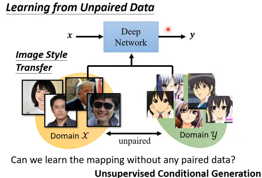
一种思路是直接使用之前的网络进行训练。将X Domain中的图像对应到Y Domain中，网络学习由X到Y的映射，然后根据输入x输出y，而分辨器根据Y Domain中的数据检验。

但很容易发现分辨器的检验是针对该图像是否为虚拟人物图像的，而非针对两者之间的对应关系。此时，当生成器认为输入图像不能从X Domain映射至Y Domain中，生成器会忽略输入x直接随机输出y；而显然分辨器并不会因为y与x无关而输出较低的值。

2. Cycle GAN

该问题曾在上节中conditional GAN上出现过，且conditional GAN可以根据paired data解决该问题，但本节并不具备该条件。

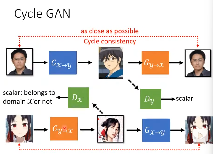
针对上述问题Cycle GAN的解决方案是训练两个生成器，一个$G_{x\to y}$学习由x到y的映射，另一个$G_{y\to x}$学习y到x的映射。

首先输入x至第一个生成器$G_{x\to y}$，生成器$G_{x\to y}$输出图像y。然后将y分别输入分辨器$D_y$和$G_{y\to x}$，前者检验生成图像是否输入X Domain，后者根据y输出图像x’。最后比对两个图像（x,x’）的相似度即可。

有想法认为，网络可能会出现直接输出原图像的旋转，而中间的图像y与x’无关。但在实作过程中，网络会较为“懒惰”的根据x输出y，很少出现该问题。但原因在理论上并没有较为详尽的解释

之后设计另一个循环，将图像y输入$G_{y\to x}$，$G_{y\to x}$输出x，x输入$D_x$和$G_{x\to y}$，$G_{x\to y}$输出y’，对比y和y’的相似度。CycleGAN由上述两个循环组成，如下图。

3. Application

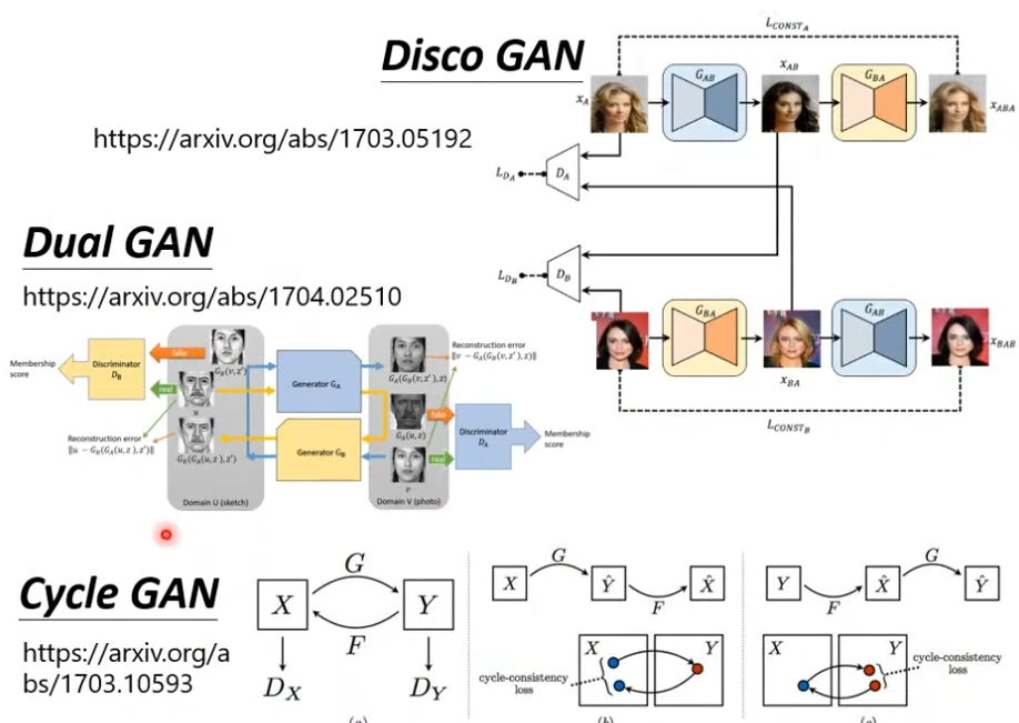
除了CycleGAN以外，还有两篇思路类似且发表日期相近的文章，链接如下。

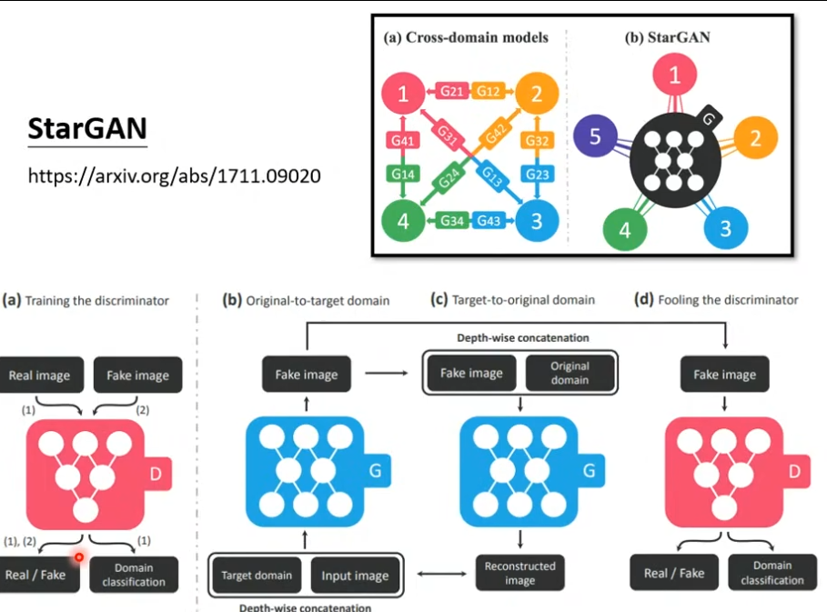
此外，还有可以做多种风格间转换的GAN，StarGAN。

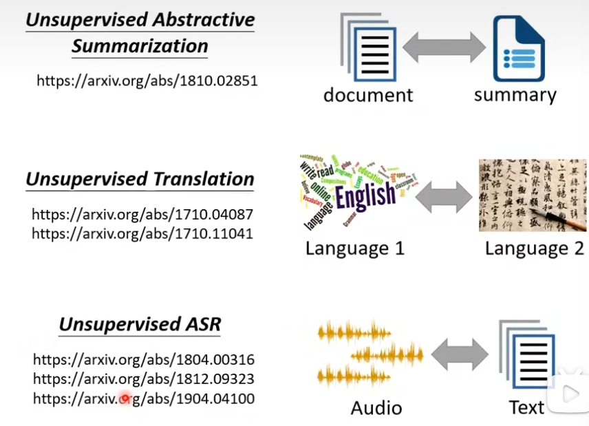
除图像风格转换外，还可以进行文字风格转换，比如将消极语句转换为积极语句，且该网络可以直接使用Cycle GAN进行训练，但分辨器需要使用RL。此外，还可用于总结、翻译、ASR等领域，具体论文如下。

二、文献阅读

1. 题目

题目：Unpaired Image-to-Image Translation using Cycle-Consistent Adversarial Networks

作者：Jun-Yan Zhu, Taesung Park, Phillip Isola, Alexei A. Efros

链接：https://arxiv.org/abs/1703.10593

发表：ICCV2017

2. abstract

该文提出了一种学习从源域到目标域映射的方法——Cycle GAN。文中将映射$G:X\to Y$与逆映射$F:Y\to X$相结合，并引入循环一致性损失(cycle consistency loss)来衡量$F(G(x))\approx X$及其反过程。最后，在非配对数据集上进行训练给出了定性结果。

This paper proposes a method for learning mapping from source domain to destination domain, namely Cycle GAN. Then this paper combines the mapping G with inverse mapping F, and introduces cycle consistency loss to measure F(G(x)) and its inverse process. Finally, this paper gives the qualitative results for training on an unpaired dataset.

3. 网络架构

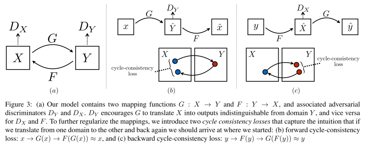
该网络的目的是学习Domain X和Y之间的映射函数，各域仅给出训练样本， { x i } i = 1 N , x i ∈ X \{x_i\}_{i=1}^N,x_i\in X {xi​}i=1N​,xi​∈X， { y j } j = 1 M , y j ∈ Y \{y_j\}_{j=1}^M,y_j\in Y {yj​}j=1M​,yj​∈Y。假定数据分布为$x\sim p_{data}(x),y\sim p_{data}(y)$。如下图所示，该网络包含两个映射$G:X\to Y,F:Y\to X$。此外，该网络引入了两个分辨器$D_X,D_Y$，其中$D_X$目标是分辨图像x和转换图像F(y)；相应的，$D_Y$目标是分表图像y和$G(x)$。

引入了两种损失计算方式。对抗性损失用于将生成图像的分布与目标域中数据分布进行匹配。循环一致性损失用于防止学习到的映射G和F相互矛盾。

3.1 损失函数

3.1.1 对抗性损失

$${\mathcal{L}}_{GAN}(G,D_Y,X,Y)={\mathbb{E}}_{y\sim p_{data}}[\log D_Y(y))]+{\mathbb{E}}_{x\sim p_{data}(x)}[\log (1-D_Y(G(x)))]$$

• y表示域Y内的样本，x表示域X内的样本
• $D_Y(y)$表示真实的Y中的样本在判别器$D_Y$之中的评分，越接近1则判别器认为此样本越真。
• G(x)为生成器根据x生成的与Y同分布的样本。
• $D_Y(G(x))$为判别器根据生成的样本得到的评分，如果DY认为生成的样本越假，则DY的评分$D_Y(G(x))$越接近于0，则 $1-D_Y(G(x))$ 越接近于1

如果判别器越强，则更能区分真实的y与生成器根据x生成的G(x)，此loss值会越大。同时，生成器希望尽可能的生成以假乱真的样本，愚弄判别器，所以生成器希望GAN loss越小。生成器与判别器在对抗的过程中，越来越强，最终生成器生成的样本以假乱真，达到判别器判别不出的程度。

$$\underset{G}{\min }\underset{D_Y}{\max }{\mathcal{L}}_{GAN}(G,D_Y,X,Y)$$
loss越大，则判别器越准确，故判别器会最大化该loss。loss越小，则声称生成样本判别器难以分辨，故分辨器会尽量最小化该loss。

3.1.2 循环一致性损失

映射函数应该是循环一致的：

• 前向循环一致性：对于来自域X的每个图像x，图像平移循环应该能够将x待会原始图像
  • 即$x\to G(x)-F(G(x))\approx x$
• 后向循环一致性：对于来自域Y的每个图像y，G和F也应满足
  • 即$y\to F(y)\to G(F(y))\approx y$

使用循环一致性损失用于激励该循环
$${\mathcal{L}}_{cyc}(G,F)={\mathbb{E}}_{x\sim p_{data}}(x)[||F(G(x))-x|{|}_1]+{\mathbb{E}}_{y\sim p_{data}}(y)[||G(F(y))-y|{|}_1]$$
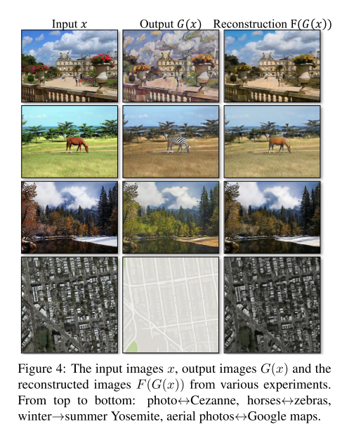
当引入循环一致性损失时，其产生的效果如下

输入图像x、输出图像G和重建图像F(G(x))

3.1.3 整体目标

综上，从而有以下综合目标
$$\mathcal{L}(G,F,D_X,D_Y)={\mathcal{L}}_{GAN}(G,D_Y,X,Y)+{\mathcal{L}}_{GAN}(F,D_X,Y,X)+\lambda {\mathcal{L}}_{cyc}(G,F)$$
其中$\lambda$控制两个目标的相关性

在上述的综合目标函数控制下，达到以下目标
$$G^{\ast },F^{\ast }=\text{arg}\underset{G,F}{\min }\underset{D_x,D_Y}{\max }\mathcal{L}(G,F,D_X,D_Y)$$

3.1.4 identity loss

在论文中应用如下parser.add_argument('--lambda_identity', type=float, default=0.5, help='use identity mapping. Setting lambda_identity other than 0 has an effect of scaling the weight of the identity mapping loss. For example, if the weight of the identity loss should be 10 times smaller than the weight of the reconstruction loss, please set lambda_identity = 0.1')
$${\mathcal{L}}_{identity}(G,F)={\mathbb{E}}_{y\sim p_{data}(y)}[||G(y)-y|{|}_1]+{\mathbb{E}}_{x\sim p_{data}(x)}[||F(x)-x|{|}_1]$$
该损失的目的是防止输入输出之间的差异过大、避免迁移过多

3.2 网络结构

采用Johnson等人的生成网络结构^[2]，判别器网络使用70*70PatchGANs

3.3 训练细节

对于loss训练，

1. 为了GAN loss${\mathcal{L}}_{GAN}(G,D,X,Y)$，训练了G以最小化${\mathbb{E}}_{x\sim p_{data}(x)}[(D(G(x))-1{)}^2]$，以及D以最小化${\mathbb{E}}_{y\sim p_{data}(y)}[(D(y)-1{)}^2]+{\mathbb{E}}_{x\sim p_{data}(x)}[D(G(x){)}^2]$
2. 为了降低模型抖动，采用了[3]

3.4 网络架构

上面介绍了网络的设计思路以及大致构成，但并没有对网络结构进行较为详细的描述，本节主要介绍该内容。

3.4.1 生成器部分

正如上文中介绍的那样，作者参照[2]设计了生成器部分的架构。该文使用6个残差块处理128$\times$128尺寸的训练图像，9个残差块处理256$\times$256尺寸的图像数据以及更高分辨率的数据。

令c7s1-k表示具有k个滤波器、步长为1的7$\times$7的Convolution-InstanceNorm-ReLU层（卷积——实例正则化——线性修正单元）。

令dk表示具有k个滤波器、步长为2的3$\times$3Convolution-InstanceNorm-ReLU层

令Rk表示残差块，其包含两个3$\times$3卷积层，两层上滤波器数量相同。

令uk表示具有k个滤波器且步长为$\frac{1}{2}$的3$\times$3fractional-strided-Convolution-InstanceNorm-ReLU层

六个残差块的网络为c7s1-64,d128,d256,R256,R256,R256,R256,R256,R256,u128,u64,c7s1-3

九个残差块的网络为c7s1-64,d128,d256,R256,R256,R256,R256,R256,R256,R256,R256,R256,u128u64,c7s1-3

3.4.2 分辨器部分

使用70$\times$70PatchGAN^[5]。

令Ck表示具有k个滤波器且步长为2的4$\times$4的Convolution-InstanceNorm-LeakyReLU层。在最后一层后，使用卷积产生一维输出。不对第一个C64层使用InstanceNorm。使用斜率为0.2的LeakyReLU层。

鉴别器架构为C64-C128-C256-C512

4. 文献解读

4.1 Introduction

该文提出了一种可以学习执行捕获一个图像集合的特殊特征，并弄清楚如何将这些特征转化为另一个图像集合，所有这些在没有任何配对训练示例的情况下进行。

假定域之间存在某种潜在关系。从两个域XY中各取一组图像，训练映射$G:X\to Y$，使得输出$\hat{y}=G(x),x\in X$。分辨器无法通过训练区分$\hat{y},y$。理论上，目标可以在$\hat{y}$上生成一个域经验分布$p_{data}(y)$相匹配的输出分布。从而最优G将Domain X转换为与Y分布相同的Domain $\hat{Y}$。但该转换并不能保证单个输入x和输出y以有意义的形式配对——存在无限多个映射G，导致$\hat{y}$上的分布相同。此外，作者在训练过程中发现难以通过单独优化对抗性目标：在一般程序上通常会导致mode collapse。

由于该问题，作者添加了更多的结构以达成目标。若有一个生成器$G:X\to Y$和另一个生成器$F:X\to Y$，则G和F应该是彼此的逆，且两个映射应该都是双射。该文通过同时训练两个映射，并添加循环一致性损失来应用这种结构假设，以激励$F(G(x))\approx x,G(F(y))\approx y$。将此损失与domain X和Y上的对抗性损失相结合，得出unpaired image dataset之间的转换。

4.2 创新点

1. 提出了一种学习从源域到目标域映射的方法——Cycle GAN
2. 引入循环一致性损失(cycle consistency loss)来衡量$F(G(x))\approx X$及其反过程
3. 在非配对数据集上进行训练给出了定性结果

4.3 实验过程

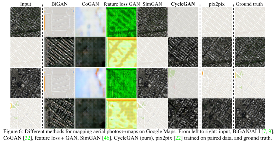
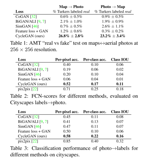
4.3.1 AMI perceptual studies地图与遥感图像迁移

4.3.2 labels-photo

FCN score(labels-photos)——Semantic segmentation metrics(photos-labels)

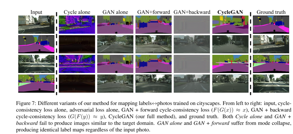
下图为cycleGAN在三个项目上的表现效果。表一：AMT。表二：FCN-scores，$labels\to photo$。表三：$photo\to labels$

相较于CoGAN, BiGAN.ALI, SimGAN, Feature loss+GAN，CycleGAN均取得了最好的效果。

4.3.3 参数设置

学习率为0.0002。D迭代两次G迭代一次。前100epoch保持相同学习率，后100epoch线性衰减至零。权重根据高斯分布$\mathcal{N}(0.02)$进行初始化

4.3.4 数据集设置

在cityscapes label与photo的训练上，使用来自[4]的2975个训练图像，图像尺寸为128$\times$128

在maps与aerial photograph上1096张训练图像从google maps上抓取，图像大小为256$\times$256。图像取自纽约市及其周边地区。然后将数据分成关于采样区域的中值纬度的训练和测试

此外该论文还使用其他多种数据集，本文仅列出与上述实验相关的部分，详见论文7.1

4.4 结论

该生成器架构是为了在外观变化上获得更好的性能而定制，并证明了在其对应领域上的最佳性能。但该任务在部分任务上表现出了故障案例，可能退化为对输入进行最小程度的改变，正如在上文中学习的那样。

三、实验内容

3.1 实验要求

基于pytorch实现GCN网络，并使用该网络基于Cora数据集进行节点分类实验

3.2 实验结果

3.3 实验代码

#%%

from torch_geometric.datasets import Planetoid

dataset = Planetoid(root='/tmp/Cora', name='Cora')


#%%

import torch
import torch.nn.functional as F
from torch_geometric.nn import GCNConv

class GCN(torch.nn.Module):
    def __init__(self):
        super().__init__()
        self.conv1 = GCNConv(dataset.num_node_features, 16)
        self.conv2 = GCNConv(16, dataset.num_classes)

    def forward(self, data):
        x, edge_index = data.x, data.edge_index

        x = self.conv1(x, edge_index)
        x = F.relu(x)
        x = F.dropout(x, training=self.training)
        x = self.conv2(x, edge_index)

        return F.log_softmax(x, dim=1)


device = torch.device('cuda' if torch.cuda.is_available() else 'cpu')
model = GCN().to(device)
data = dataset[0].to(device)
optimizer = torch.optim.Adam(model.parameters(), lr=0.01, weight_decay=5e-4)

model.train()
for epoch in range(200):
    optimizer.zero_grad()
    out = model(data)
    loss = F.nll_loss(out[data.train_mask], data.y[data.train_mask])
    loss.backward()
    optimizer.step()

#%%

model.eval()
pred = model(data).argmax(dim=1)
correct = (pred[data.test_mask] == data.y[data.test_mask]).sum()
acc = int(correct) / int(data.test_mask.sum())
print(f'Accuracy: {acc:.4f}')

3.4 其他相关代码

CycleGAN

#%% md

<a href="https://colab.research.google.com/github/bkkaggle/pytorch-CycleGAN-and-pix2pix/blob/master/CycleGAN.ipynb" target="_parent"><img src="https://colab.research.google.com/assets/colab-badge.svg" alt="Open In Colab"/></a>

#%% md

Take a look at the [repository](https://github.com/junyanz/pytorch-CycleGAN-and-pix2pix) for more information

#%% md

# Install

#%%

!git clone https://github.com/junyanz/pytorch-CycleGAN-and-pix2pix

#%%

import os
os.chdir('pytorch-CycleGAN-and-pix2pix/')

#%%

!pip install -r requirements.txt

#%% md

# Datasets

Download one of the official datasets with:

-   `bash ./datasets/download_cyclegan_dataset.sh [apple2orange, summer2winter_yosemite, horse2zebra, monet2photo, cezanne2photo, ukiyoe2photo, vangogh2photo, maps, cityscapes, facades, iphone2dslr_flower, ae_photos]`

Or use your own dataset by creating the appropriate folders and adding in the images.

-   Create a dataset folder under `/dataset` for your dataset.
-   Create subfolders `testA`, `testB`, `trainA`, and `trainB` under your dataset's folder. Place any images you want to transform from a to b (cat2dog) in the `testA` folder, images you want to transform from b to a (dog2cat) in the `testB` folder, and do the same for the `trainA` and `trainB` folders.

#%%

!bash ./datasets/download_cyclegan_dataset.sh horse2zebra

#%% md

# Pretrained models

Download one of the official pretrained models with:

-   `bash ./scripts/download_cyclegan_model.sh [apple2orange, orange2apple, summer2winter_yosemite, winter2summer_yosemite, horse2zebra, zebra2horse, monet2photo, style_monet, style_cezanne, style_ukiyoe, style_vangogh, sat2map, map2sat, cityscapes_photo2label, cityscapes_label2photo, facades_photo2label, facades_label2photo, iphone2dslr_flower]`

Or add your own pretrained model to `./checkpoints/{NAME}_pretrained/latest_net_G.pt`

#%%

!bash ./scripts/download_cyclegan_model.sh horse2zebra

#%% md

# Training

-   `python train.py --dataroot ./datasets/horse2zebra --name horse2zebra --model cycle_gan`

Change the `--dataroot` and `--name` to your own dataset's path and model's name. Use `--gpu_ids 0,1,..` to train on multiple GPUs and `--batch_size` to change the batch size. I've found that a batch size of 16 fits onto 4 V100s and can finish training an epoch in ~90s.

Once your model has trained, copy over the last checkpoint to a format that the testing model can automatically detect:

Use `cp ./checkpoints/horse2zebra/latest_net_G_A.pth ./checkpoints/horse2zebra/latest_net_G.pth` if you want to transform images from class A to class B and `cp ./checkpoints/horse2zebra/latest_net_G_B.pth ./checkpoints/horse2zebra/latest_net_G.pth` if you want to transform images from class B to class A.


#%%

!python train.py --dataroot ./datasets/horse2zebra --name horse2zebra --model cycle_gan --display_id -1

#%% md

# Testing

-   `python test.py --dataroot datasets/horse2zebra/testA --name horse2zebra_pretrained --model test --no_dropout`

Change the `--dataroot` and `--name` to be consistent with your trained model's configuration.

> from https://github.com/junyanz/pytorch-CycleGAN-and-pix2pix:
> The option --model test is used for generating results of CycleGAN only for one side. This option will automatically set --dataset_mode single, which only loads the images from one set. On the contrary, using --model cycle_gan requires loading and generating results in both directions, which is sometimes unnecessary. The results will be saved at ./results/. Use --results_dir {directory_path_to_save_result} to specify the results directory.

> For your own experiments, you might want to specify --netG, --norm, --no_dropout to match the generator architecture of the trained model.

#%%

!python test.py --dataroot datasets/horse2zebra/testA --name horse2zebra_pretrained --model test --no_dropout

#%% md

# Visualize

#%%

import matplotlib.pyplot as plt

img = plt.imread('./results/horse2zebra_pretrained/test_latest/images/n02381460_1010_fake.png')
plt.imshow(img)

#%%

import matplotlib.pyplot as plt

img = plt.imread('./results/horse2zebra_pretrained/test_latest/images/n02381460_1010_real.png')
plt.imshow(img)

CycleGANModel

import torch
import itertools
from util.image_pool import ImagePool
from .base_model import BaseModel
from . import networks


class CycleGANModel(BaseModel):
    """
    This class implements the CycleGAN model, for learning image-to-image translation without paired data.

    The model training requires '--dataset_mode unaligned' dataset.
    By default, it uses a '--netG resnet_9blocks' ResNet generator,
    a '--netD basic' discriminator (PatchGAN introduced by pix2pix),
    and a least-square GANs objective ('--gan_mode lsgan').

    CycleGAN paper: https://arxiv.org/pdf/1703.10593.pdf
    """
    @staticmethod
    def modify_commandline_options(parser, is_train=True):
        """Add new dataset-specific options, and rewrite default values for existing options.

        Parameters:
            parser          -- original option parser
            is_train (bool) -- whether training phase or test phase. You can use this flag to add training-specific or test-specific options.

        Returns:
            the modified parser.

        For CycleGAN, in addition to GAN losses, we introduce lambda_A, lambda_B, and lambda_identity for the following losses.
        A (source domain), B (target domain).
        Generators: G_A: A -> B; G_B: B -> A.
        Discriminators: D_A: G_A(A) vs. B; D_B: G_B(B) vs. A.
        Forward cycle loss:  lambda_A * ||G_B(G_A(A)) - A|| (Eqn. (2) in the paper)
        Backward cycle loss: lambda_B * ||G_A(G_B(B)) - B|| (Eqn. (2) in the paper)
        Identity loss (optional): lambda_identity * (||G_A(B) - B|| * lambda_B + ||G_B(A) - A|| * lambda_A) (Sec 5.2 "Photo generation from paintings" in the paper)
        Dropout is not used in the original CycleGAN paper.
        """
        parser.set_defaults(no_dropout=True)  # default CycleGAN did not use dropout
        if is_train:
            parser.add_argument('--lambda_A', type=float, default=10.0, help='weight for cycle loss (A -> B -> A)')
            parser.add_argument('--lambda_B', type=float, default=10.0, help='weight for cycle loss (B -> A -> B)')
            parser.add_argument('--lambda_identity', type=float, default=0.5, help='use identity mapping. Setting lambda_identity other than 0 has an effect of scaling the weight of the identity mapping loss. For example, if the weight of the identity loss should be 10 times smaller than the weight of the reconstruction loss, please set lambda_identity = 0.1')

        return parser

    def __init__(self, opt):
        """Initialize the CycleGAN class.

        Parameters:
            opt (Option class)-- stores all the experiment flags; needs to be a subclass of BaseOptions
        """
        BaseModel.__init__(self, opt)
        # specify the training losses you want to print out. The training/test scripts will call <BaseModel.get_current_losses>
        self.loss_names = ['D_A', 'G_A', 'cycle_A', 'idt_A', 'D_B', 'G_B', 'cycle_B', 'idt_B']
        # specify the images you want to save/display. The training/test scripts will call <BaseModel.get_current_visuals>
        visual_names_A = ['real_A', 'fake_B', 'rec_A']
        visual_names_B = ['real_B', 'fake_A', 'rec_B']
        if self.isTrain and self.opt.lambda_identity > 0.0:  # if identity loss is used, we also visualize idt_B=G_A(B) ad idt_A=G_A(B)
            visual_names_A.append('idt_B')
            visual_names_B.append('idt_A')

        self.visual_names = visual_names_A + visual_names_B  # combine visualizations for A and B
        # specify the models you want to save to the disk. The training/test scripts will call <BaseModel.save_networks> and <BaseModel.load_networks>.
        if self.isTrain:
            self.model_names = ['G_A', 'G_B', 'D_A', 'D_B']
        else:  # during test time, only load Gs
            self.model_names = ['G_A', 'G_B']

        # define networks (both Generators and discriminators)
        # The naming is different from those used in the paper.
        # Code (vs. paper): G_A (G), G_B (F), D_A (D_Y), D_B (D_X)
        self.netG_A = networks.define_G(opt.input_nc, opt.output_nc, opt.ngf, opt.netG, opt.norm,
                                        not opt.no_dropout, opt.init_type, opt.init_gain, self.gpu_ids)
        self.netG_B = networks.define_G(opt.output_nc, opt.input_nc, opt.ngf, opt.netG, opt.norm,
                                        not opt.no_dropout, opt.init_type, opt.init_gain, self.gpu_ids)

        if self.isTrain:  # define discriminators
            self.netD_A = networks.define_D(opt.output_nc, opt.ndf, opt.netD,
                                            opt.n_layers_D, opt.norm, opt.init_type, opt.init_gain, self.gpu_ids)
            self.netD_B = networks.define_D(opt.input_nc, opt.ndf, opt.netD,
                                            opt.n_layers_D, opt.norm, opt.init_type, opt.init_gain, self.gpu_ids)

        if self.isTrain:
            if opt.lambda_identity > 0.0:  # only works when input and output images have the same number of channels
                assert(opt.input_nc == opt.output_nc)
            self.fake_A_pool = ImagePool(opt.pool_size)  # create image buffer to store previously generated images
            self.fake_B_pool = ImagePool(opt.pool_size)  # create image buffer to store previously generated images
            # define loss functions
            self.criterionGAN = networks.GANLoss(opt.gan_mode).to(self.device)  # define GAN loss.
            self.criterionCycle = torch.nn.L1Loss()
            self.criterionIdt = torch.nn.L1Loss()
            # initialize optimizers; schedulers will be automatically created by function <BaseModel.setup>.
            self.optimizer_G = torch.optim.Adam(itertools.chain(self.netG_A.parameters(), self.netG_B.parameters()), lr=opt.lr, betas=(opt.beta1, 0.999))
            self.optimizer_D = torch.optim.Adam(itertools.chain(self.netD_A.parameters(), self.netD_B.parameters()), lr=opt.lr, betas=(opt.beta1, 0.999))
            self.optimizers.append(self.optimizer_G)
            self.optimizers.append(self.optimizer_D)

    def set_input(self, input):
        """Unpack input data from the dataloader and perform necessary pre-processing steps.

        Parameters:
            input (dict): include the data itself and its metadata information.

        The option 'direction' can be used to swap domain A and domain B.
        """
        AtoB = self.opt.direction == 'AtoB'
        self.real_A = input['A' if AtoB else 'B'].to(self.device)
        self.real_B = input['B' if AtoB else 'A'].to(self.device)
        self.image_paths = input['A_paths' if AtoB else 'B_paths']

    def forward(self):
        """Run forward pass; called by both functions <optimize_parameters> and <test>."""
        self.fake_B = self.netG_A(self.real_A)  # G_A(A)
        self.rec_A = self.netG_B(self.fake_B)   # G_B(G_A(A))
        self.fake_A = self.netG_B(self.real_B)  # G_B(B)
        self.rec_B = self.netG_A(self.fake_A)   # G_A(G_B(B))

    def backward_D_basic(self, netD, real, fake):
        """Calculate GAN loss for the discriminator

        Parameters:
            netD (network)      -- the discriminator D
            real (tensor array) -- real images
            fake (tensor array) -- images generated by a generator

        Return the discriminator loss.
        We also call loss_D.backward() to calculate the gradients.
        """
        # Real
        pred_real = netD(real)
        loss_D_real = self.criterionGAN(pred_real, True)
        # Fake
        pred_fake = netD(fake.detach())
        loss_D_fake = self.criterionGAN(pred_fake, False)
        # Combined loss and calculate gradients
        loss_D = (loss_D_real + loss_D_fake) * 0.5
        loss_D.backward()
        return loss_D

    def backward_D_A(self):
        """Calculate GAN loss for discriminator D_A"""
        fake_B = self.fake_B_pool.query(self.fake_B)
        self.loss_D_A = self.backward_D_basic(self.netD_A, self.real_B, fake_B)

    def backward_D_B(self):
        """Calculate GAN loss for discriminator D_B"""
        fake_A = self.fake_A_pool.query(self.fake_A)
        self.loss_D_B = self.backward_D_basic(self.netD_B, self.real_A, fake_A)

    def backward_G(self):
        """Calculate the loss for generators G_A and G_B"""
        lambda_idt = self.opt.lambda_identity
        lambda_A = self.opt.lambda_A
        lambda_B = self.opt.lambda_B
        # Identity loss
        if lambda_idt > 0:
            # G_A should be identity if real_B is fed: ||G_A(B) - B||
            self.idt_A = self.netG_A(self.real_B)
            self.loss_idt_A = self.criterionIdt(self.idt_A, self.real_B) * lambda_B * lambda_idt
            # G_B should be identity if real_A is fed: ||G_B(A) - A||
            self.idt_B = self.netG_B(self.real_A)
            self.loss_idt_B = self.criterionIdt(self.idt_B, self.real_A) * lambda_A * lambda_idt
        else:
            self.loss_idt_A = 0
            self.loss_idt_B = 0

        # GAN loss D_A(G_A(A))
        self.loss_G_A = self.criterionGAN(self.netD_A(self.fake_B), True)
        # GAN loss D_B(G_B(B))
        self.loss_G_B = self.criterionGAN(self.netD_B(self.fake_A), True)
        # Forward cycle loss || G_B(G_A(A)) - A||
        self.loss_cycle_A = self.criterionCycle(self.rec_A, self.real_A) * lambda_A
        # Backward cycle loss || G_A(G_B(B)) - B||
        self.loss_cycle_B = self.criterionCycle(self.rec_B, self.real_B) * lambda_B
        # combined loss and calculate gradients
        self.loss_G = self.loss_G_A + self.loss_G_B + self.loss_cycle_A + self.loss_cycle_B + self.loss_idt_A + self.loss_idt_B
        self.loss_G.backward()

    def optimize_parameters(self):
        """Calculate losses, gradients, and update network weights; called in every training iteration"""
        # forward
        self.forward()      # compute fake images and reconstruction images.
        # G_A and G_B
        self.set_requires_grad([self.netD_A, self.netD_B], False)  # Ds require no gradients when optimizing Gs
        self.optimizer_G.zero_grad()  # set G_A and G_B's gradients to zero
        self.backward_G()             # calculate gradients for G_A and G_B
        self.optimizer_G.step()       # update G_A and G_B's weights
        # D_A and D_B
        self.set_requires_grad([self.netD_A, self.netD_B], True)
        self.optimizer_D.zero_grad()   # set D_A and D_B's gradients to zero
        self.backward_D_A()      # calculate gradients for D_A
        self.backward_D_B()      # calculate graidents for D_B
        self.optimizer_D.step()  # update D_A and D_B's weights

小结

本周学习了上周简要介绍的Conditional GAN，并主要学习了CycleGAN网络结构。该网络基于两个映射$F:X\to Y,G:Y\to Y$构造了两个循环$X\to Y\to X^{\prime },Y\to X\to Y^{\prime }$，并设计了两个分辨器$D_X,D_Y$分别用于检测两个生成器伪造的X、Y图像是否为假。为了避免整个循环差异过大，引入了循环一致性检测。尽管在小部分情况下，可能出现网络在循环后生成的图像相较于循环前仅有较小的改变，且中间伪造的另一个数据集的图像与输入数据相关性不大；但总的来说该网络可以较好的训练并得出针对非配对数据集间的映射。下周将简要学习自监督学习。

参考文献

[1] Zhu, Jun-Yan, et al. “Unpaired Image-to-Image Translation Using Cycle-Consistent Adversarial Networks.” arXiv.Org, 24 Aug. 2020, arxiv.org/abs/1703.10593.

[2] J. Johnson, A. Alahi, and L. Fei-Fei. Perceptual losses for real-time style transfer and super-resolution. In ECCV, 2016. 2, 3, 5, 7, 18

[3] A. Shrivastava, T. Pfister, O. Tuzel, J. Susskind, W. Wang, and R. Webb. Learning from simulated and unsupervised images through adversarial training. In CVPR, 2017

[4] M. Cordts, M. Omran, S. Ramos, T. Rehfeld, M. Enzweiler, R. Benenson, U. Franke, S. Roth, and B. Schiele. The cityscapes dataset for semantic urban scene understanding. In CVPR, 2016. 2, 5, 6, 18

[5] P. Isola, J.-Y. Zhu, T. Zhou, and A. A. Efros. Image-to-image translation with conditional adversarial networks. In CVPR, 2017. 2, 3, 5, 6, 7, 8, 18