李宏毅机器学习第二十四周周报 Self-attention ConvLSTM

week 24 Self-attention ConvLSTM for Spatiotemporal Prediction

摘要

本文主要讨论SA ConvLSTM的模型。本文简要介绍了LSTM的结构以及运行逻辑，并展示了ConvLSTM。其次本文展示了题为Self-Attention ConvLSTM for Spatiotemporal Prediction的论文主要内容。这篇论文提出了Self-attention ConvLSTM模型，该模型将自注意力机制引入到 ConvLSTM 中。具体来说，提出了一种新颖的自注意力记忆（SAM）来记忆在空间和时间域方面具有远程依赖性的特征。该文在多个数据集上进行实验，从数据角度证明了该网络的优越性。最后，本文基于pytorch实现了GRU和LSTM模型并用于预测时序数据集的后续结果。

Abstract

This article focuses on SA ConvLSTM. This article briefly describes the structure and operation logic of LSTM, and shows the ConvLSTM. Secondly, this paper presents the main content of the paper entitled Self-Attention ConvLSTM for Spatiotemporal Prediction. This paper proposes self-attention ConvLSTM model, which introduces the self-attention mechanism into ConvLSTM. Specifically, a novel self-attention memory (SAM) is proposed to memorize features that are remotely dependent in terms of spatial and temporal domains. This paper carries out experiments on several datasets, and the proves superiority of the network from the perspective of data. Finally, this article implements the GRU and LSTM model based on pytorch and uses them to predict the subsequent results of time series datasets.

一、机器学习

为了便于文献的阅读，以下简要介绍LSTM以及ConvLSTM

下图为LSTM的内部结构图，该结构可以通过级联形成神经网络

二、文献阅读

1. 题目

题目：Self-Attention ConvLSTM for Spatiotemporal Prediction

作者：Zhihui Lin, Maomao Li, Zhuobin Zheng, Yangyang Cheng, Chun Yuan

链接：https://doi.org/10.1609/aaai.v34i07.6819

发布：Vol. 34 No. 07: AAAI-20 Technical Tracks 7 /AAAI Technical Track: Vision

2. abstract

为了提取具有全局和局部依赖性的空间特征，将自注意力机制引入到 ConvLSTM 中。具体来说，提出了一种新颖的自注意力记忆（SAM）来记忆在空间和时间域方面具有远程依赖性的特征。基于自注意力，SAM 可以通过聚合输入本身所有位置的特征和具有成对相似度分数的记忆特征来生成特征。此外，将 SAM 嵌入到标准 ConvLSTM 中，构建用于时空预测的自注意力 ConvLSTM（SA-ConvLSTM）。在实验中，应用SA-ConvLSTM对MovingMNIST和KTH数据集进行帧预测，对TexiBJ数据集进行交通流预测。

To extract spatial features with both global and local dependencies, authors introduce the self-attention mechanism into ConvLSTM. Specifically, a novel self-attention memory (SAM) is proposed to memorize features with long-range dependencies in terms of spatial and temporal domains. Based on the self-attention, SAM can produce features by aggregating features across all positions of both the input itself and memory features with pair-wise similarity scores. Furthermore, authors embed the SAM into a standard ConvLSTM to construct a self-attention ConvLSTM (SA-ConvLSTM) for the spatiotemporal prediction. In experiments, authors apply the SA-ConvLSTM to perform frame prediction on the MovingMNIST and KTH datasets and traffic flow prediction on the TexiBJ dataset.

3. 网络架构

为了评估 self-attention 在时空预测中的有效性，通过级联 self-attention 模块和标准 ConvLSTM 构建了一个基本的 self-attention ConvLSTM 模型。随后，基于所提出的自注意力记忆模块构建了更先进和复杂的模型 SAConvLSTM。

3.1基础模型

Self-Attetion：下图显示了标准自注意力模型的流程。原始图${\mathcal{H}}_t$被映射至不同的特征空间作为查询query：${\mathbf{Q}}_h={\mathbf{W}}_q{\mathcal{H}}_t\in {\mathbb{R}}^{\hat{C}\times N}$，键key：${\mathbf{K}}_h={\mathbf{W}}_k{\mathcal{H}}_t\in {\mathbb{R}}^{\hat{C}\times N}$，以及值key：${\mathbf{V}}_h={\mathbf{W}}_v{\mathcal{H}}_t\in R^{C\times N}$，其中 { W q , W k , W v } \{\mathbf W_q, \mathbf W_k, \mathbf W_v\} {Wq​,Wk​,Wv​}是一个$1\times 1$卷积层的权重集，$C,\hat{C}$是通道数，其中$N=H\times W$。每对点的相似度通过应用矩阵产生式来计算：
$$\mathbf{e}={\mathbf{Q}}_h^T{\mathbf{K}}_h\in {\mathbb{R}}^{N\times N}\text{\hspace{1em}(2)}$$

上图为标准自注意力模块和建议的自注意力内存模块（简称 SAM）的图示。在自注意力模块中，${\mathcal{H}}_t$是时间步t处ConvLSTM中的隐藏状态，${\mathbf{Q}}_h$是查询，${\mathbf{K}}_h$表示键，${\mathbf{V}}_h$表示基于特征上的1×1卷积的值，${\hat{\mathcal{H}}}_t$是输出。对于所提出的SAM，聚合特征${\mathbf{Z}}_h$是通过对Ht和另一个特征${\mathbf{Z}}_m$应用自注意力来获得的，其中${\mathbf{Z}}_m$是通过查询${\mathbf{K}}_m$并访问${\mathbf{V}}_m$来计算的。这里，${\mathbf{K}}_m$和${\mathbf{V}}_m$都是存储器${\mathcal{M}}_{t-1}$的映射。 ${\mathbf{Z}}_h$和${\mathbf{Z}}_m$通过1×1卷积融合为Z。然后使用 Z 和原始输入 ${\mathcal{H}}_t$ 通过门控机制更新内存。最终输出是输出门值和更新后的内存${\mathcal{M}}_t$​之间的点积。

第 i 个点和第 j 个点之间的相似度可以索引为 $e_{i,j}=({\mathcal{H}}_{t,i}^T{\mathbf{W}}_q^T)({\mathbf{W}}_k{\mathcal{H}}_{t,j})$ 其中 $H_{t,i}$ 和 $H_{t,j}$ 是具有以下形状的特征向量C × 1。然后，相似度分数沿列标准化：
α i , j = exp ⁡ e i , j ∑ k = 1 N exp ⁡ e i , k , i , j ∈ { 1 , 2 , … , N } (3) \alpha_{i,j}=\frac{\exp e_{i,j}}{\sum_{k=1}^N\exp e_{i,k}},i,j\in \{1,2,\dots,N\} \tag{3} αi,j​=∑k=1N​expei,k​expei,j​​,i,j∈{1,2,…,N}(3)
第 i 个位置的聚合特征是通过所有位置的加权和来计算的：
$${\mathbf{Z}}_i=\sum _{j=1}^N{\alpha }_{i,j}({\mathbf{W}}_v{\mathcal{H}}_{t;j})\text{\hspace{1em}(4)}$$
其中${\mathbf{W}}_v{\mathcal{H}}_{t,j}\in {\mathbb{R}}^{C\times 1}$ 是值 ${\mathbf{V}}_h$ 的第 j 列。输出是通过快捷连接 ${\mathcal{H}}_t={\mathbf{W}}_f\mathbf{Z}+{\mathcal{H}}_t$ 获得的。这里，残差机制稳定了模型训练，并确保模块可以灵活地嵌入到其他深度模型中。

3.2自注意力记忆模块

认为当前时间步长的预测可以受益于过去的相关特征。因此通过构建具有自注意力机制的新设计的记忆单元M，提出了自注意力记忆模块。使用所提出的记忆单元来表示具有全局空间和时间感受野的一般时空信息。

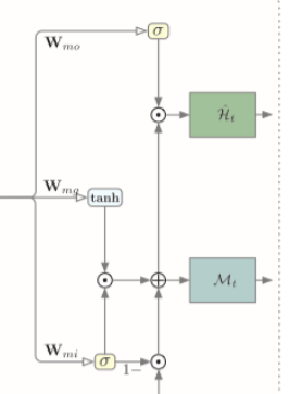
下图为自注意力记忆模块，其接受两个输入，当前时间步的输入特征 ${\mathcal{H}}_t$ 和最后一步的记忆 ${\mathcal{M}}_{t-1}$。整个流程可以分为三个部分：特征聚合以获得全局上下文信息、内存更新和输出。

特征聚合。在每个时间步，聚合特征 $\mathbf{Z}$ 是 ${\mathbf{Z}}_h$ 和 ${\mathbf{Z}}_m$ 的融合。 ${\mathbf{Z}}_m$ 通过在最后一个时间步 ${\mathcal{M}}_{t-1}$ 查询内存来聚合。内存通过权重 ${\mathbf{W}}_{mk}$ 和 ${\mathbf{W}}_{mv}$ 通过 1 × 1 卷积映射为键 ${\mathbf{K}}_m\in {\mathbb{R}}^{\hat{C}\times N}$ 和值 ${\mathbf{V}}_m\in {\mathbb{R}}^{C\times N}$。然后，通过查询 ${\mathbf{Q}}_h$ 和密钥 ${\mathbf{K}}_m$ 之间的矩阵乘法计算输入和内存之间的相似度分数：
$${\mathbf{e}}_m={\mathbf{Q}}_h^T{\mathbf{K}}_m\in {\mathbb{R}}^{N\times N}\text{\hspace{1em}(5)}$$
用于聚合特征的所有权重都是通过沿每行应用 SoftMax 函数获得的，故有和（3）类似的以下等式：
α m ; i , j = exp ⁡ e m ; i , j ∑ k = 1 N exp ⁡ e m ; i , k , i , j ∈ { 1 , 2 , … , N } (6) \alpha_{m;i,j}=\frac{\exp e_{m;i,j}}{\sum_{k=1}^N\exp e_{m;i,k}},i,j\in\{1,2,\dots,N\} \tag{6} αm;i,j​=∑k=1N​expem;i,k​expem;i,j​​,i,j∈{1,2,…,N}(6)
然后，特征 ${\mathbf{Z}}_m$ 中第 i 个位置的“像素”通过值 ${\mathbf{V}}_m$ 中所有 N 个位置的加权和来计算
$${\mathbf{Z}}_{m;i}=\sum _{j=1}^N{\alpha }_{m;i,j}{\mathbf{V}}_{m;j}=\sum _{j=1}^N{\alpha }_{m;i,j}{\mathbf{W}}_{mv}{\mathcal{M}}_{t-1;j}\text{\hspace{1em}(7)}$$
其中${\mathcal{M}}_{t-1}$是第j列的记忆。

最后，聚合特征$\mathbf{Z}$可由$\mathbf{Z}={\mathbf{W}}_z[{\mathbf{Z}}_h;{\mathbf{Z}}_m]$​获得

内存更新。采用门控机制自适应的更新内存M，使得SAM可以捕获时空域的长程依赖性。聚合特征Z和原始输入${\mathcal{H}}_t$用于生成输入们$i_t$以及融合特征$g_t$。更新进度可以表述为：
$$\begin{gathered} i_t^{\prime }=\sigma (W_{m;zi}\ast \mathbf{Z}+W_{m;hi}\ast {\mathcal{H}}_t+b_{m;i}) \\ {g}_t^{\prime }=\text{tanh}(W_{m;zg}\ast \mathbf{Z}+W_{m;hg}\ast {\mathcal{H}}_t+b_{m;g}) \\ {\mathcal{M}}_t=(1-i_t^{\prime })\circ {\mathcal{M}}_{t-1}+i_t^{\prime }\circ g_t^{\prime }\text{\hspace{1em}(8)} \end{gathered}$$

输出。自注意力记忆模块的输出特征 ${\hat{\mathcal{H}}}_t$​ 是输出门 o t 与更新记忆 Mt 之间的点积，可以表示为：
$$o_t^{\prime }=\sigma (W_{m;zo}\ast \mathbf{Z}+W_{m;ho}\ast {\mathcal{H}}_t+b_{m;o}){\hat{\mathcal{H}}}_t=o_t^{\prime }\circ {\mathcal{M}}_t\text{\hspace{1em}(9)}$$

3.3Self-Attention ConvLSTM

SAM是3.2中描述的框架，作者将该部分嵌入到ConvLSTM中。相应的，SAM可以灵活的嵌入到其他模型。

4. 文献解读

4.1 Introduction

由于复杂的动力学和外观变化，时空预测具有挑战性。其中，一个关键问题是如何让ConvLSTM捕获有效的长程依赖关系。作者认为当前时间步长的特征可以从过去聚合相关特征中受益。因此，该文提出了 ConvLSTM 的自注意力记忆模块，简称 SAM。 SAM利用自注意力的特征聚合机制，通过计算成对相似度得分来融合当前特征和记忆特征。将 SAM 嵌入到 ConvLSTM 中，构建自注意力 ConvLSTM，简称 SA-ConvLSTM。消融实验证明了自我关注和额外记忆对不同类型数据的有效性。此外，SA-ConvLSTM 在所有数据集上以比以前最先进的方法更少的参数和更高的效率实现了最佳结果。

4.2 创新点

1. 提出了 ConvLSTM 的一种新变体，名为 SAConvLSTM 来执行时空预测，它可以成功捕获远程空间依赖性。
2. 设计了一个基于记忆的自注意力模块（SAM）来记住预测过程中的全局时空依赖性。
3. 在 MovingMNIST 和 KTH 上评估 SA-ConvLSTM 进行多帧预测，在 TexiBJ 上评估交通流预测。与当前最先进的模型 MIM 相比，它以更少的参数和更高的效率在所有数据集中取得了最佳结果。

4.3 实验过程

使用三个常用数据集进行时空预测，包含 MovingMNIST 和 KTH上进行多帧预测，以及TexiBJ上的交通流预测。首先对 MovingMNIST 和 TexiBJ 进行消融研究。随后，展示了每个数据集的定量结果。

4.3.1实现

应用了具有 64 个隐藏状态的 4 层架构每个模型的每一层。训练过程中采用了预定采样策略和层标准化。每个模型都使用 ADAM 优化器进行训练，初始学习率为 0.001。训练时，小批量设置为8，训练过程在80,000次迭代后停止。对 MovingMNIST 和 TaxiBJ 数据集使用 L2 损失，对 KTH 数据集使用 L1+ L2 损失。

4.3.2数据集

MovingMNIST：描绘了两个可能重叠的数字以恒定速度移动并从图像边缘反弹。图像大小为64×64×1，每个序列包含20帧，其中10个输入和10个用于预测。

TaxiBJ：从混乱的现实环境中收集的，包含从北京出租车的GPS监视器连续收集的交通流图像。每一帧都是 32 × 32 × 2 的图像网格。两个通道代表此时进出同一小区的车流量。我们使用 4 个已知帧来预测接下来的 4 帧

KTH：包含 6 类人类动作，包括拳击、挥手、拍手、行走、慢跑和跑步，由 25 个人在 4 个不同场景中完成。图像大小从 320×240 调整为 128×128。10 帧用于在训练期间预测接下来的 10 帧，在推理时预测接下来的 20 帧。

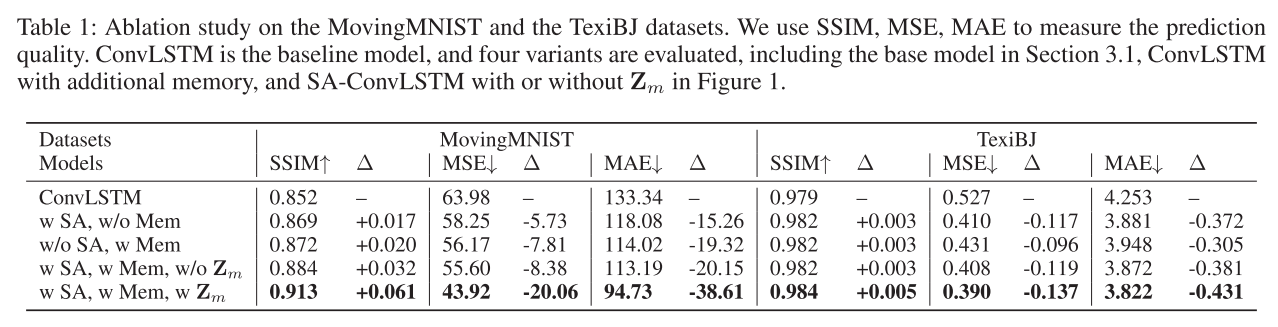
4.3.3消融实验

MovingMNIST 和 TexiBJ 进行了消融研究，以评估不同类型数据的模型。

应用了五种不同的模型：

1. 标准的4层ConvLSTM
2. 如图2所示构建的带有自注意力的基本模型
3. 带有额外记忆单元M但没有自注意力部分的ConvLSTM
4. 图1中没有${\mathbf{Z}}_m$的SA-ConvLSTM
5. 完整的SA-ConvLSTM

采用SSIM（结构相似性指数度量）、MSE（均方误差）和MAE（平均绝对误差）作为度量，其中MSE和MAE测量像素级差异。

实验结果如下表所示。整个SA-ConvLSTM结合了两者的优点，在这两类数据上分别降低了32.2%和26.0%的MSE。从具有全局空间和时间依赖性的附加记忆中聚合过去的特征对于 SA-ConvLSTM 来说非常重要。

4.3.4定量以及定性实验

MovingMNIST：PredRNN、PredRNN++、MIM等模型作为比较。所有模型都根据之前 10 帧预测接下来的 10 帧。该模型做出了其中较好的成果，且模型规模相较于其他模型具有一定优势。定性结果如下表

TaxiBJ：下表为该数据集测试集的定量比较。每个模型通过 4 个已知帧预测接下来的 4 帧。采用逐帧 MSE 作为度量。所提出的 SA-ConvLSTM 比 MIM 降低了平均 MSE 误差约 9.3%。

KTH。下表显示了 KTH 数据集的定量比较结果。使用最后 10 帧来预测接下来的 20 帧。 SA-ConvLSTM在KTH数据集上展示了其高效率和灵活性。它相较于最先进模型的 PSNR 提高了 0.86，SSIM 提高了 0.026。基础模型仍然取得了与 PredRNN 相当的结果。SA Conv-LSTM不仅可以保留更多的纹理信息，而且可以提高预测精度。

4.3.5注意力可视化

为了解释所提出的 SA-ConvLSTM 中自注意力机制的效果，我们从 MovingMNIST 的测试集中随机选择一些示例，并将注意力图可视化，如下图所示，其中注意力图为

颜色越暖的区域与查询点的相关性越强。当查询点位于背景上时，大部分权重集中在背景上。低层（第1层）特征是平移不变的，使得背景特征基本相同，第1层可以统一关注背景像素。相比之下，第 4 层的特征具有更多语义信息。这里，Moving-MNIST 中数字出现在角落的概率非常低。这种统计先验可以由网络学习。SAM 学习将角点处的特征转换为背景滤波器，这可用于构建更准确的前景或背景特征。

4.4 结论

在本文中，提出了用于时空预测的 SA-ConvLSTM。由于当前时间步的预测可以受益于过去的相关特征，因此我们构建了一个自注意力记忆模块来捕获空间和时间维度上的远程依赖性。与之前最先进的模型相比，所提出的 SA-ConvLSTM 在所有数据集上以更少的参数和更高的效率实现了最佳结果。

三、使用GRU和LSTM进行时间预测

使用的数据集是每小时能源消耗数据集，可以在Kaggle上找到。该数据集包含按小时记录的美国不同地区的电力消耗数据，链接地址

目标是创建一个模型，可以根据历史使用数据准确预测下一小时的能源使用情况。使用 GRU 和 LSTM 模型来训练一组历史数据，并在未见过的测试集上评估这两个模型。从特征选择和数据预处理开始，然后定义、训练并最终评估模型。

1.库的导入&数据集

import os
import time

import numpy as np
import pandas as pd
import matplotlib.pyplot as plt

import torch
import torch.nn as nn
from torch.utils.data import TensorDataset, DataLoader

from tqdm import tqdm_notebook
from sklearn.preprocessing import MinMaxScaler

# Define data root directory
data_dir = "./data/"
print(os.listdir(data_dir))

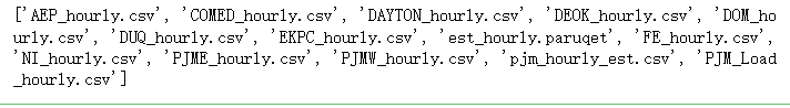
以上为本实验所使用的数据集

pd.read_csv(data_dir + 'AEP_hourly.csv').head()

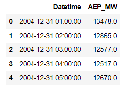
数据集规格如上图

2.数据预处理

按以下顺序读取这些文件并预处理这些数据：

• 获取每个单独时间步的时间数据并对它们进行概括
  • 一天中的某个小时，即 0 - 23
  • 一周中的某一天，即。1 - 7
  • 月份，即 1 - 12
  • 一年中的某一天，即 1 - 365
• 将数据缩放到 0 到 1 之间的值
  • 当特征具有相对相似的规模和/或接近正态分布时，算法往往会表现更好或收敛得更快
  • 缩放保留了原始分布的形状并且不会降低异常值的重要性
• 将数据分组为序列，用作模型的输入并存储其相应的标签
  • 序列长度或回顾周期是模型用于进行预测的历史数据点的数量
  • 标签将是输入序列中最后一个数据点之后的下一个数据点
• 将输入和标签拆分为训练集和测试集

# The scaler objects will be stored in this dictionary so that our output test data from the model can be re-scaled during evaluation
label_scalers = {}

train_x = []
test_x = {}
test_y = {}

for file in tqdm_notebook(os.listdir(data_dir)): 
    # Skipping the files we're not using
    if file[-4:] != ".csv" or file == "pjm_hourly_est.csv":
        continue
    
    # Store csv file in a Pandas DataFrame
    df = pd.read_csv('{}/{}'.format(data_dir, file), parse_dates=[0])
    # Processing the time data into suitable input formats
    df['hour'] = df.apply(lambda x: x['Datetime'].hour,axis=1)
    df['dayofweek'] = df.apply(lambda x: x['Datetime'].dayofweek,axis=1)
    df['month'] = df.apply(lambda x: x['Datetime'].month,axis=1)
    df['dayofyear'] = df.apply(lambda x: x['Datetime'].dayofyear,axis=1)
    df = df.sort_values("Datetime").drop("Datetime",axis=1)
    
    # Scaling the input data
    sc = MinMaxScaler()
    label_sc = MinMaxScaler()
    data = sc.fit_transform(df.values)
    # Obtaining the Scale for the labels(usage data) so that output can be re-scaled to actual value during evaluation
    label_sc.fit(df.iloc[:,0].values.reshape(-1,1))
    label_scalers[file] = label_sc
    
    # Define lookback period and split inputs/labels
    lookback = 90
    inputs = np.zeros((len(data)-lookback,lookback,df.shape[1]))
    labels = np.zeros(len(data)-lookback)
    
    for i in range(lookback, len(data)):
        inputs[i-lookback] = data[i-lookback:i]
        labels[i-lookback] = data[i,0]
    inputs = inputs.reshape(-1,lookback,df.shape[1])
    labels = labels.reshape(-1,1)
    
    # Split data into train/test portions and combining all data from different files into a single array
    test_portion = int(0.1*len(inputs))
    if len(train_x) == 0:
        train_x = inputs[:-test_portion]
        train_y = labels[:-test_portion]
    else:
        train_x = np.concatenate((train_x,inputs[:-test_portion]))
        train_y = np.concatenate((train_y,labels[:-test_portion]))
    test_x[file] = (inputs[-test_portion:])
    test_y[file] = (labels[-test_portion:])

数据规模print(train_x.shape):(980185, 90, 5)

为了提高训练速度，批量处理数据，这样模型就不需要频繁更新权重。Torch Dataset和DataLoader类对于将数据拆分为批次并对其进行混洗非常有用。

batch_size = 1024
train_data = TensorDataset(torch.from_numpy(train_x), torch.from_numpy(train_y))
train_loader = DataLoader(train_data, shuffle=True, batch_size=batch_size, drop_last=True)

使用gpu训练

# torch.cuda.is_available() checks and returns a Boolean True if a GPU is available, else it'll return False
is_cuda = torch.cuda.is_available()

# If we have a GPU available, we'll set our device to GPU. We'll use this device variable later in our code.
if is_cuda:
    device = torch.device("cuda")
else:
    device = torch.device("cpu")

3.模型定义

定义GRU以及LSTM模型

class GRUNet(nn.Module):
    def __init__(self, input_dim, hidden_dim, output_dim, n_layers, drop_prob=0.2):
        super(GRUNet, self).__init__()
        self.hidden_dim = hidden_dim
        self.n_layers = n_layers
        
        self.gru = nn.GRU(input_dim, hidden_dim, n_layers, batch_first=True, dropout=drop_prob)
        self.fc = nn.Linear(hidden_dim, output_dim)
        self.relu = nn.ReLU()
        
    def forward(self, x, h):
        out, h = self.gru(x, h)
        out = self.fc(self.relu(out[:,-1]))
        return out, h
    
    def init_hidden(self, batch_size):
        weight = next(self.parameters()).data
        hidden = weight.new(self.n_layers, batch_size, self.hidden_dim).zero_().to(device)
        return hidden

class LSTMNet(nn.Module):
    def __init__(self, input_dim, hidden_dim, output_dim, n_layers, drop_prob=0.2):
        super(LSTMNet, self).__init__()
        self.hidden_dim = hidden_dim
        self.n_layers = n_layers
        
        self.lstm = nn.LSTM(input_dim, hidden_dim, n_layers, batch_first=True, dropout=drop_prob)
        self.fc = nn.Linear(hidden_dim, output_dim)
        self.relu = nn.ReLU()
        
    def forward(self, x, h):
        out, h = self.lstm(x, h)
        out = self.fc(self.relu(out[:,-1]))
        return out, h
    
    def init_hidden(self, batch_size):
        weight = next(self.parameters()).data
        hidden = (weight.new(self.n_layers, batch_size, self.hidden_dim).zero_().to(device),
                  weight.new(self.n_layers, batch_size, self.hidden_dim).zero_().to(device))
        return hidden

两个模型在隐藏状态和层中将具有相同数量的维度，在相同数量的epoch和学习率上进行训练，并在完全相同的数据集上进行训练和测试。

将使用对称平均绝对百分比误差(SMAPE)来评估模型
KaTeX parse error: Unexpected end of input in a macro argument, expected '}' at end of input: …y_i|+|y_i|)/2}

4.训练过程

def train(train_loader, learn_rate, hidden_dim=256, EPOCHS=5, model_type="GRU"):
    
    # Setting common hyperparameters
    input_dim = next(iter(train_loader))[0].shape[2]
    output_dim = 1
    n_layers = 2
    # Instantiating the models
    if model_type == "GRU":
        model = GRUNet(input_dim, hidden_dim, output_dim, n_layers)
    else:
        model = LSTMNet(input_dim, hidden_dim, output_dim, n_layers)
    model.to(device)
    
    # Defining loss function and optimizer
    criterion = nn.MSELoss()
    optimizer = torch.optim.Adam(model.parameters(), lr=learn_rate)
    
    model.train()
    print("Starting Training of {} model".format(model_type))
    epoch_times = []
    # Start training loop
    for epoch in range(1,EPOCHS+1):
        start_time = time.perf_counter()
        h = model.init_hidden(batch_size)
        avg_loss = 0.
        counter = 0
        for x, label in train_loader:
            counter += 1
            if model_type == "GRU":
                h = h.data
            else:
                h = tuple([e.data for e in h])
            model.zero_grad()
            
            out, h = model(x.to(device).float(), h)
            loss = criterion(out, label.to(device).float())
            loss.backward()
            optimizer.step()
            avg_loss += loss.item()
            if counter%200 == 0:
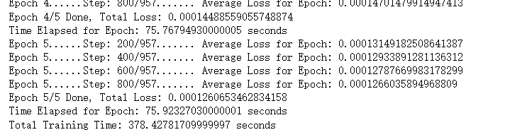
                print("Epoch {}......Step: {}/{}....... Average Loss for Epoch: {}".format(epoch, counter, len(train_loader), avg_loss/counter))
        current_time = time.perf_counter()
        print("Epoch {}/{} Done, Total Loss: {}".format(epoch, EPOCHS, avg_loss/len(train_loader)))
        print("Time Elapsed for Epoch: {} seconds".format(str(current_time-start_time)))
        epoch_times.append(current_time-start_time)
    print("Total Training Time: {} seconds".format(str(sum(epoch_times))))
    return model

def evaluate(model, test_x, test_y, label_scalers):
    model.eval()
    outputs = []
    targets = []
    start_time = time.perf_counter()
    for i in test_x.keys():
        inp = torch.from_numpy(np.array(test_x[i]))
        labs = torch.from_numpy(np.array(test_y[i]))
        h = model.init_hidden(inp.shape[0])
        out, h = model(inp.to(device).float(), h)
        outputs.append(label_scalers[i].inverse_transform(out.cpu().detach().numpy()).reshape(-1))
        targets.append(label_scalers[i].inverse_transform(labs.numpy()).reshape(-1))
    print("Evaluation Time: {}".format(str(time.perf_counter()-start_time)))
    sMAPE = 0
    for i in range(len(outputs)):
        sMAPE += np.mean(abs(outputs[i]-targets[i])/(targets[i]+outputs[i])/2)/len(outputs)
    print("sMAPE: {}%".format(sMAPE*100))
    return outputs, targets, sMAPE
#time模块在Python 3.x版本中已经将clock()方法废弃。应该使用time.perf_counter()或者time.process_time()方法来代替clock()

5.模型训练

lr = 0.001
gru_model = train(train_loader, lr, model_type="GRU")

lstm_model = train(train_loader, lr, model_type="LSTM")

使用SMAPE评估模型

gru_outputs, targets, gru_sMAPE = evaluate(gru_model, test_x, test_y, label_scalers):

Evaluation Time: 26.02710079999997
sMAPE: 0.33592208657162453%

lstm_outputs, targets, lstm_sMAPE = evaluate(lstm_model, test_x, test_y, label_scalers):

Evaluation Time: 19.92910290000009
sMAPE: 0.38698768153562335%

两者性能相近，lstm较优，但是并没有明显的区别

小结

本周主要复习了LSTM结构，并简要了解了ConvLSTM作为论文阅读的前导。随后，本文阅读了SA ConvLSTM。最后实现了LSTM和GRU。下周预计阅读ConvLSTM

参考文献

[1] Lin, Zhihui, et al. “Self-Attention CONVLSTM for Spatiotemporal Prediction.” Proceedings of the AAAI Conference on Artificial Intelligence, ojs.aaai.org/index.php/AAAI/article/view/6819. Accessed 4 Jan. 2020.