机器学习之集成学习-随机森林篇（二）

一、前文回顾

《机器学习之集成学习-概述篇（一）》概述了集成学习是多学习器的强强联合，指出了集成学习具有更好的泛化性、准确性，了解了集成分类的两种方式：bagging和bootsting。本文对集成分类中的bagging集成分类进行剖析并取其典型随机森林算法，进行知识讲解及案例分析。

二、Bagging算法原理

Bagging顾名思义，背包，背袋。它取自统计学习里面随机抽样，从一个未知样本集中有放回的抽取数据。假设有m个样本，随机取出一个样本放入采样集中，然后再将样本放回初始数据集中，这样该样本仍有可能被选中，经过m次随机采样，得到m个样本的采样集。

初始训练中的数据集有的在样本中出现过，有的从未出现过，这样我们采样出T个含m个训练样本的采样集，然后基于每个采样集训练出一个基学习器，再将这些基学器进行结合，这就是Bagging的基本流程。

**Bagging示意图**

按照少数服从多数的原则产生预测结果。

分类任务一般采用投票法，回归任务一般采用平均法。

结论：1、初始样本集中有63.2%的样本出现在采样集中。

2、偏差-方差分解的角度，主要关注降低方差，因此在不剪枝决策树、神经网络等易受样本扰动的学习器上效用更明显。

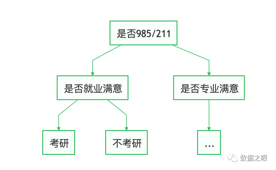
三、决策树算法原理

决策树，顾名思义是基于树结构来进行决策的，是我们面临决策问题时一种很自然的处理机制，最终结论对应我们希望的判定结果。

一般讲，一棵决策树包含一个根结点、若干内部节点和若干叶节点，叶节点对应决策结果，其他节点则对应属性测试；每个节点包含的样本集合根据属性测试的结果被划分到子节点中；根节点包含样本全集。根节点到叶节点对应一个判定测试序列。决策树示例图：

**决策树示意图**

四、随机森林算法原理

随机森林(Random Forest,简称RF)，是Bagging的一个扩展变体，其弱学习器是决策树模型。

**随机森林示意图**

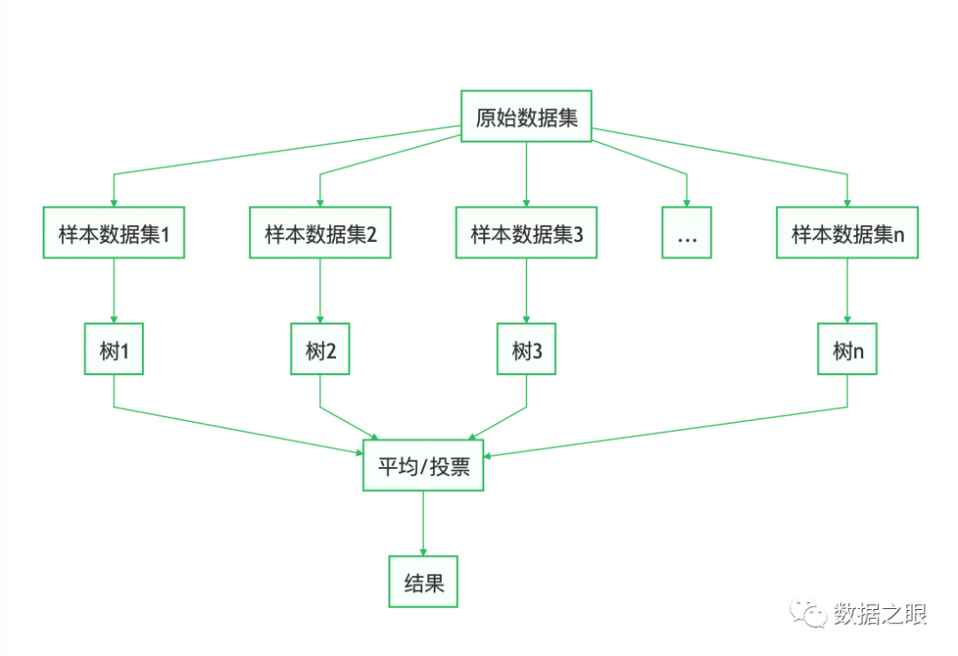
随机森林会在原始数据集中随机抽取数据，然后构成n个不同的样本集，根据这些数据集搭建n个不同的决策树模型，最后根据这些决策树模型的平均值（回归模型）或者投票情况（分类模型）获取最终结果。为保证模型泛化能力，减少过拟合，它遵循数据随机和特征随机两个原则。

1、数据随机，即样本扰动。遵循bagging算法原理，从原始数据集中有放回的采样出n个弱学习需要的训练数据集。

2、特征随机，即属性扰动。

传统决策树：在选择划分属性时，是在当前结点的属性集合(假定有d个属性)中选择一个最优属性。

随机森林：RF在以决策树为基学习器构建Bagging集成的基础上，进一步在决策树训练过程中引入随机属性选择。对决策树的每个节点，先从该节点的属性结合中随机选择一个包含k个属性的子集，然后再从这个子集中选择一个最优属性用于划分。

K控制了随机性的引入程度：若令K=d,则基决策树的构建与传统决策树相同。若令K=1，则是随机选择一个属性用于划分；一般情况下，推荐值k=log2d，python中默认值为根号d。

五、随机森林案例

# -*- coding: utf-8 -*-
import pandas as pd
import matplotlib.pyplot as plt
import seaborn as sns
from sklearn.model_selection import train_test_split
from sklearn.ensemble import RandomForestClassifier
from sklearn.metrics import classification_report
import numpy as np
from sklearn.model_selection import GridSearchCV  # 网格搜索
#第一步：获取数据，并清洗数据
# 1、读取数据
data = pd.read_csv('bank.csv', sep=';', encoding='utf-8')
data = data[data.columns]
print(data)
#第二步:数据分析，找寻数据之间的关系
# 2、计算皮尔逊相关系数
plt.figure(figsize=(20, 20))
plt.rcParams['font.sans-serif'] = ['SimHei']
plt.rcParams['axes.unicode_minus'] = False
sns.heatmap(data.corr(), cmap="YlGnBu", annot=True)
plt.title("相关性分析图")
plt.show()
#第三步：数据转换，将数据转换成模型中可以应用的数据
# 3、转换数据类型将字符串类型转成大于0的数字
data['job'] = pd.factorize(data['job'])[0].astype(int)
data['marital'] = pd.factorize(data['marital'])[0].astype(int)
data['education'] = pd.factorize(data['education'])[0].astype(int)
data['default'] = pd.factorize(data['default'])[0].astype(int)
data['housing'] = pd.factorize(data['housing'])[0].astype(int)
data['loan'] = pd.factorize(data['loan'])[0].astype(int)
data['contact'] = pd.factorize(data['contact'])[0].astype(int)
data['month'] = pd.factorize(data['month'])[0].astype(int)
data['poutcome'] = pd.factorize(data['poutcome'])[0].astype(int)
data['y'] = pd.factorize(data['y'])[0].astype(int)
print(data)
#第四步：数据建模，划分测试集与训练集
# 4、划分测试集与训练集
x = data.iloc[:, :-1]
y = data['y']
X_train, X_test, y_train, y_test = train_test_split(x, y, random_state=90)
# 5、随机森林模型
model = RandomForestClassifier()  # 建立默认参数的模型
# 训练模型
model.fit(X_train, y_train)
# 预测值
y_pred = model.predict(X_test)

#第五步：模型评估，计算各种情况下模型的准确率
# 求出预测和真实一样的数目
true = np.sum(y_pred == y_test)
print('预测对的结果数目为：', true)
print('预测错的的结果数目为：', y_test.shape[0] - true)
# 评估指标
from sklearn.metrics import accuracy_score, precision_score, recall_score, f1_score, cohen_kappa_score

# 准确率（针对所有的预测类型）：预测为对（预测和真实一样）的样本数/预测的总样本数
print('预测数据的准确率为：{:.4}%'.format(accuracy_score(y_test, y_pred) * 100))
# 精确率（针对某个预测类型，找对了多少）：预测为A正确的样本数/（预测为A正确的样本+预测A错误的样本数）
print('预测数据的精确率为：{:.4}%'.format(precision_score(y_test, y_pred) * 100))
# 召回率（针对某个预测类型，找全了多少）：预测为A正确的样本数/（预测为A正确的样本+预测B错误的样本数）
print('预测数据的召回率为：{:.4}%'.format(recall_score(y_test, y_pred) * 100))
# F1:F1 Score = 2*（P*R）/ (P+R)，其中P和R分别为 precision 和recall。
# 精确率分母：预测为A正确的样本数；召回率的分母：原来样本就是A的样本数
print('预测数据的F1值为：', f1_score(y_test, y_pred))
print('预测数据的Cohen’s Kappa系数为：', cohen_kappa_score(y_test, y_pred))
# 打印分类报告
print('预测数据的分类报告为：', '\n', classification_report(y_test, y_pred))
#第六步：模型参数调优
# 6、参数调优
#利用GridSearchCV进行参数调优，
#GridSearchCV:拆分为成GridSearch和CV，即网格搜索和交叉验证。网格搜索，搜索的是参数，
# 即在指定的参数范围内，按步长依次调整参数，利用调整的参数训练学习器，从所有的参数中找到在
# 验证集上精度最高的参数，这其实是一个训练和比较的过程。
# 6-1、按树进行调优:n_estimators  '种树'（树的数量）
scorel = []
for i in range(0, 200, 10):
    model = RandomForestClassifier(n_estimators=i + 1,
                                   n_jobs=-1,
                                   random_state=90).fit(X_train, y_train)
    score = model.score(X_test, y_test)
    scorel.append(score)
# 最大值对应的索引值：
print("max:", max(scorel),
      (scorel.index(max(scorel)) * 10) + 1)  # 作图反映出准确度随着估计器数量的变化，71的附近最好
plt.figure(figsize=[20, 5])
plt.plot(range(1, 201, 10), scorel)
plt.show()
## 6-2、根据上面的显示最优点在90附近，进一步细化学习曲线
scorel = []
for i in range(85, 100):
    RFC = RandomForestClassifier(n_estimators=i, n_jobs=-1,
                                 random_state=90).fit(X_train, y_train)
    score = RFC.score(X_test, y_test)
    scorel.append(score)

print(max(scorel),
      ([*range(85, 100)][scorel.index(max(scorel))]))  # 76是最优的估计器数量
plt.figure(figsize=[20, 5])
plt.plot(range(85, 100), scorel)
plt.show()
##6-3：树的最大深度优化
scorel = []
for i in range(3, 30):
    RFC = RandomForestClassifier(max_depth=i,
                                 n_estimators=89,
                                 n_jobs=-1,
                                 random_state=90).fit(X_train, y_train)
    score = RFC.score(X_test, y_test)
    scorel.append(score)

print(max(scorel), ([*range(3, 30)][scorel.index(max(scorel))]))
plt.figure(figsize=[20, 5])
plt.plot(range(3, 30), scorel)
plt.show()
# 树的最大深度（max_depth）默认可以不输入，
# 在数据量较大或者特征较多的时候可以限制在10-100之间避免模型太复杂导致过拟合，
# 如果数据量较小或特征不多的情况下是可以不输入的，比如此处数据量也不是很大，可以不用调整
##6-4：最小叶子优化
scorel = []
for i in range(1, 20):
    RFC = RandomForestClassifier(max_depth=28,
                                 n_estimators=89,
                                 min_samples_leaf=i,
                                 n_jobs=-1,
                                 random_state=90).fit(X_train, y_train)
    score = RFC.score(X_test, y_test)
    scorel.append(score)

print(max(scorel), ([*range(1, 20)][scorel.index(max(scorel))]))
plt.figure(figsize=[20, 5])
plt.plot(range(1, 20), scorel)
plt.show()
##6-5：最大特征优化
## 调整max_features
param_grid = {'max_features': ['auto', 'sqrt', 'log2']}
RFC = RandomForestClassifier(max_depth=28,
                             n_estimators=89,
                             min_samples_leaf=1,
                             min_samples_split=6)
GS = GridSearchCV(RFC, param_grid, cv=10)
GS.fit(X_train, y_train)
print(GS.best_params_)  # 最佳最大特征方法：auto
print(GS.best_score_)

##6-6、criterion优化
param_grid = {'criterion': ['gini', 'entropy']}
RFC = RandomForestClassifier(max_depth=28,
                             n_estimators=89,
                             min_samples_leaf=1,
                             min_samples_split=6,
                             max_features='auto')
GS = GridSearchCV(RFC, param_grid, cv=10)
GS.fit(X_train, y_train)
print(GS.best_params_)
print(GS.best_score_)
##6-7、min_samples_leaf 优化
param_grid = {'min_samples_leaf': np.arange(1, 11, 1)}
RFC = RandomForestClassifier(max_depth=28,
                             n_estimators=89,
                             min_samples_leaf=1,
                             min_samples_split=6,
                             max_features='auto',
                             criterion='entropy')
GS = GridSearchCV(RFC, param_grid, cv=10)
GS.fit(X_train, y_train)
print(GS.best_params_)
print(GS.best_score_)
##6-8、最终结果评估
feat_labels = data.columns[:-1]
# n_jobs  整数 可选（默认=1） 适合和预测并行运行的作业数，如果为-1，则将作业数设置为核心数
RFC = RandomForestClassifier(max_depth=28,
                             n_estimators=89,
                             min_samples_leaf=6,
                             min_samples_split=7,
                             max_features='auto',
                             criterion='entropy',
                             random_state=0,
                             n_jobs=-1)
RFC.fit(X_train, y_train)
labe_name = []
imports = []

# 下面对训练好的随机森林，完成重要性评估
# feature_importances_  可以调取关于特征重要程度
importances = RFC.feature_importances_
print("重要性：", importances)
x_columns = data.columns[:-1]
#argsort排序是从小到大的，因此要用[::-1]进行倒序，得到从大到小的排序。
#按数值从小到大排序，取排序之前数值对应的索引值即列的下标号
indices = np.argsort(importances)[::-1]
for f in range(X_train.shape[1]):
    # 对于最后需要逆序排序，我认为是做了类似决策树回溯的取值，从叶子收敛
    # 到根，根部重要程度高于叶子。
    print("%2d) %-*s %f" %
          (f + 1, 30, feat_labels[indices[f]], importances[indices[f]]))
    labe_name.append(feat_labels[indices[f]])
    imports.append(importances[indices[f]])

# 构造数据
a = pd.DataFrame({"feature": labe_name})
b = pd.DataFrame({"importance": imports})
df = pd.concat([a, b], axis=1)

# 特征重要性柱状图
plt.figure(figsize=(100, 100))
plt.rcParams['font.sans-serif'] = ['SimHei']
plt.rcParams['axes.unicode_minus'] = False
sns.barplot(x="importance",
            y="feature",
            data=df,
            order=df["feature"],
            orient="h")
plt.show()

六、写在文末

本文是自学笔记，有需要可以借鉴，关于更细致的知识点会形成自己的知识百科点。